
# Insertion Loss and Trace Width: A Practical Guide for High-Frequency PCB Design
At low frequencies, a PCB trace is a wire. At high frequencies, it is a transmission line, and transmission lines lose energy. This energy loss, quantified as insertion loss in decibels per unit length, determines whether a signal arrives with enough amplitude to be correctly received. For Indian teams designing 5G infrastructure, military radar, satellite communications, and high-speed serial links, managing insertion loss is the difference between a board that works and one that does not.
As Indian industry pushes into mmWave 5G (Jio, Airtel), X-band radar (Indian defence agencies), and interfaces like PCIe Gen5 and 112G SerDes, the design choices that control insertion loss, trace width, copper roughness, dielectric material, and stackup geometry, must be made early, informed by simulation rather than rules of thumb. This article provides a practical guide to the physics, design parameters, and Siemens EDA tools, HyperLynx SI and Z Planner, that enable Indian teams to optimise their high-frequency designs.
Why Insertion Loss Matters
A signal travelling through a PCB trace loses amplitude as it propagates. If insertion loss is too high, the eye diagram closes, voltage and timing margins shrink until the receiver cannot distinguish logic levels. At 1 Gbps on a 15 cm trace, FR-4 is manageable. At 10 Gbps, insertion loss becomes a significant constraint. At 28 Gbps, standard FR-4 may make the channel non-functional.
High-frequency PCB design requires explicit management of insertion loss through material selection, trace geometry, and stackup design, decisions that must be made during board planning and validated through simulation before routing begins.
The Physics of Insertion Loss
Insertion loss in a PCB trace has three primary components, each with distinct frequency dependence:
Conductor Loss (Skin Effect)
At DC, current flows uniformly through the trace cross-section. As frequency increases, current crowds toward the surface, the skin effect. At 1 GHz, skin depth is approximately 2.1 micrometres; at 10 GHz, approximately 0.66 micrometres. Current flows through an increasingly thin shell, effectively increasing resistance.
Wider traces have lower conductor loss because the current-carrying perimeter is longer. A 200-micrometre trace has roughly twice the conducting perimeter of a 100-micrometre trace, and therefore roughly half the conductor loss. However, wider traces require thicker dielectric to maintain impedance, increasing board thickness, a tradeoff requiring simulation to optimise.
Dielectric Loss
The dielectric material absorbs electromagnetic energy, characterised by its dissipation factor (Df). FR-4 has Df of approximately 0.02 at 1 GHz. Low-loss materials like Megtron 6 achieve 0.002 or less, an order of magnitude improvement.
Dielectric loss increases approximately linearly with frequency and overtakes conductor loss between 3-8 GHz for most configurations. Above a few gigahertz, material selection has more impact on insertion loss than copper geometry. Indian teams designing 5G mmWave, Ku-band satellite links, or 56G/112G SerDes channels cannot use standard FR-4.
Copper Roughness Loss
This loss mechanism catches many engineers by surprise. Copper foil has a deliberate roughness profile for dielectric adhesion, invisible at low frequencies but significant when skin depth approaches roughness height. Roughness is characterised by the Rz value (average peak-to-valley height):
- Standard (STD) copper: Rz approximately 6-10 micrometres
- Low-profile (LP) copper: Rz approximately 3-5 micrometres
- Very low-profile (VLP) copper: Rz approximately 1.5-3 micrometres
- Hyper very low-profile (HVLP) copper: Rz approximately 1-2 micrometres
At 10 GHz, when skin depth (0.66 micrometres) is comparable to roughness features, current follows the rough contour, increasing path length and resistance. The difference between standard and VLP copper can be 0.5-1.0 dB per inch at 10 GHz, significant over a 10-20 inch channel. For Indian teams designing above 10 GHz, copper roughness is a primary design variable.
Trace Width: The Direct Lever
Trace width is the most directly controllable parameter affecting conductor loss. Halving trace width roughly doubles conductor loss. But width cannot be considered in isolation, trace width and dielectric thickness together determine characteristic impedance (typically 50 ohms single-ended, 85-100 ohms differential).
This creates a design optimisation problem:
- Narrower trace, thinner dielectric: Higher conductor loss, but thinner stackup, more routing layers possible
- Wider trace, thicker dielectric: Lower conductor loss, but thicker stackup, fewer routing layers
The optimal trace width depends on target frequency, channel length, board thickness constraints, available materials, and loss budget, precisely the multi-variable optimisation that simulation tools solve.
Dielectric Material Selection
For Indian teams working at frequencies above 3-5 GHz, the choice of dielectric material is the single most impactful decision for insertion loss management. The spectrum of available materials ranges from standard FR-4 to ultra-low-loss materials, with corresponding differences in performance and cost:
Standard FR-4 (Dk ~4.3, Df ~0.02 at 1 GHz). Adequate for designs operating below 2-3 GHz. Widely available from Indian PCB fabricators. Cost-effective. Not suitable for high-frequency or long-channel high-speed serial links. Mid-loss materials (Dk ~3.6-3.8, Df ~0.008-0.012). Materials like Megtron 4 and similar mid-loss laminates provide a significant improvement over FR-4 at a moderate cost premium. Suitable for PCIe Gen4, 25G Ethernet, and similar mid-frequency applications. Low-loss materials (Dk ~3.3-3.6, Df ~0.002-0.005). Materials like Megtron 6 and Rogers RO4000 series are used for demanding high-frequency applications. Required for PCIe Gen5, 56G SerDes, and 5G sub-6 GHz systems. Available from specialised fabricators. Ultra-low-loss materials (Dk ~3.0-3.5, Df <0.002). Materials like Rogers RO3000 series and similar PTFE-based laminates are used for mmWave, radar, and satellite applications. Required for 28 GHz 5G, X-band radar, and Ku-band satellite systems. Limited fabricator availability in India, most Indian teams source these boards from specialised international fabricators or the few domestic facilities with mmWave capability.
Material choice must be validated through simulation. HyperLynx SI models frequency-dependent dielectric properties, allowing engineers to compare materials and select the most cost-effective option meeting the loss budget.
Z Planner: Stackup Optimisation
Z Planner allows engineers to define the PCB stackup, copper weights, dielectric materials, thicknesses, and roughness profiles, and calculate resulting impedance and insertion loss. It addresses the fundamental problem of balancing impedance targets with loss budgets:
- Characteristic impedance for single-ended and differential traces at specified widths and spacings
- Insertion loss per unit length as a function of frequency, accounting for conductor loss, dielectric loss, and copper roughness
- Stackup thickness and its impact on board manufacturability and mechanical requirements
An Indian team designing a 5G base station backplane, for example, might use Z Planner to evaluate several stackup options:
- Standard FR-4 with 1 oz copper and standard roughness, lowest cost, highest loss
- Megtron 6 with 1 oz LP copper, moderate cost, significantly lower loss
- Megtron 6 with 0.5 oz HVLP copper and wider traces, higher cost, lowest loss
Z Planner quantifies the insertion loss for each option across the frequency range of interest, enabling an informed engineering decision rather than a guess.
HyperLynx SI: Channel Simulation
HyperLynx SI provides the simulation engine for validating high-frequency signal integrity on the actual PCB layout. Key capabilities for insertion loss management include:
S-Parameter Analysis
S-parameters characterise frequency-dependent behaviour including insertion loss (S21), return loss (S11), and crosstalk. HyperLynx SI extracts S-parameters from PCB layout geometry, accounting for trace width, dielectric properties, copper roughness, via transitions, and connectors.
For Indian radar and satellite teams, S-parameter analysis is the primary validation tool. An X-band radar front-end must maintain insertion loss across 8-12 GHz, HyperLynx SI models these transitions using actual geometry and material properties.
Channel Simulation
For high-speed serial links, HyperLynx SI cascades S-parameters of each channel segment, traces, vias, connectors, cables, and evaluates overall performance against the interface specification, accounting for all loss mechanisms and producing a realistic loss budget assessment.
Eye Diagrams with Realistic Loss Models
HyperLynx SI generates eye diagrams incorporating frequency-dependent insertion loss and transmitter/receiver equalisation (pre-emphasis, CTLE, DFE). For Indian teams designing PCIe Gen5 or 100G Ethernet, this simulation confirms the design will work, or identifies problems while changes are still possible.
Indian Applications
The need for insertion loss management spans several critical Indian industry segments:
5G Infrastructure. Jio and Airtel are deploying mmWave bands at 26-28 GHz. Base station antenna feed networks, beamforming arrays, and backhaul interfaces all require insertion loss management at frequencies where FR-4 is inadequate. Military Radar. Indian defence agencies and OEMs develop radar systems from L-band through Ku-band. At X-band and above, every decibel of feed network loss reduces detection range. Material selection, trace geometry, and stackup must minimise loss at the operating frequency. Satellite Communications. ISRO’s programmes, including NavIC and broadband satellite constellations, require ground terminal and payload electronics achieving specified insertion loss targets across L-band through Ku-band. High-Speed Digital. Indian companies working with advanced processors encounter PCIe Gen4/Gen5, DDR5, USB4, and 100G/400G Ethernet, where insertion loss management is essential for first-pass success.
A Methodology, Not Just a Tool
Managing insertion loss in high-frequency PCB design is not a single analysis step, it is a methodology that spans the entire design process:
1. Requirements definition: Establish the loss budget for each critical channel based on the interface specification and the transmitter/receiver capabilities
2. Material selection: Use Z Planner to evaluate dielectric materials and copper roughness profiles against the loss budget
3. Stackup optimisation: Use Z Planner to determine trace widths, dielectric thicknesses, and layer assignments that meet both impedance and loss targets
4. Layout implementation: Route critical channels in Xpedition with the constraints defined during stackup optimisation
5. Channel validation: Use HyperLynx SI to extract S-parameters, simulate the complete channel, and generate eye diagrams
6. Iteration: If the channel does not meet its loss budget, adjust the material, stackup, or routing, informed by simulation rather than guesswork
This methodology ensures that insertion loss is managed proactively throughout the design, rather than discovered as a problem during board bring-up.
Getting Started with GSAS
GSAS Micro Systems provides high-frequency design methodology support for Indian teams, from stackup planning and material selection through channel simulation and validation.
Contact GSAS Micro Systems today for high-frequency design methodology support. Whether you are designing 5G infrastructure, military radar, satellite communications, or high-speed digital systems, GSAS can help you establish the insertion loss management methodology that ensures first-pass success. Our field application engineers are based in Bengaluru, Hyderabad, Chennai, Coimbatore, Pune, and Delhi NCR. Reach us through gsasindia.com or visit our offices in Bengaluru, Chennai, or Vadodara.
Also appears in:
Interested in Siemens EDA tools?
Talk to our application engineers for personalized tool recommendations.
More from Siemens EDA
View all →
India's EDA Moment: Why Design Tool Demand Is Growing, and the Engineering Careers It Creates
21 Sept · 9 min

AI and Complexity Are Redrawing EDA: Siemens on the Trillion-Transistor Era
13 Sept · 6 min
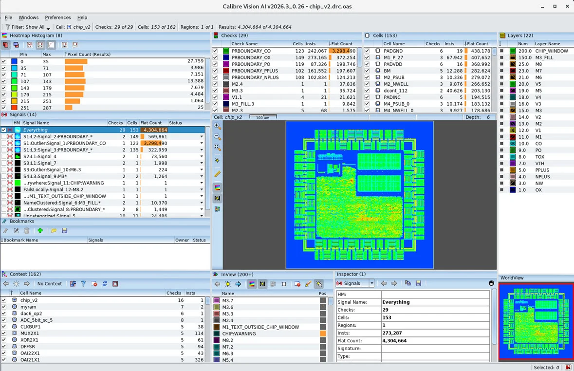
Calibre Vision AI: Bringing Order to DRC Debug at Advanced Nodes
24 Aug · 4 min
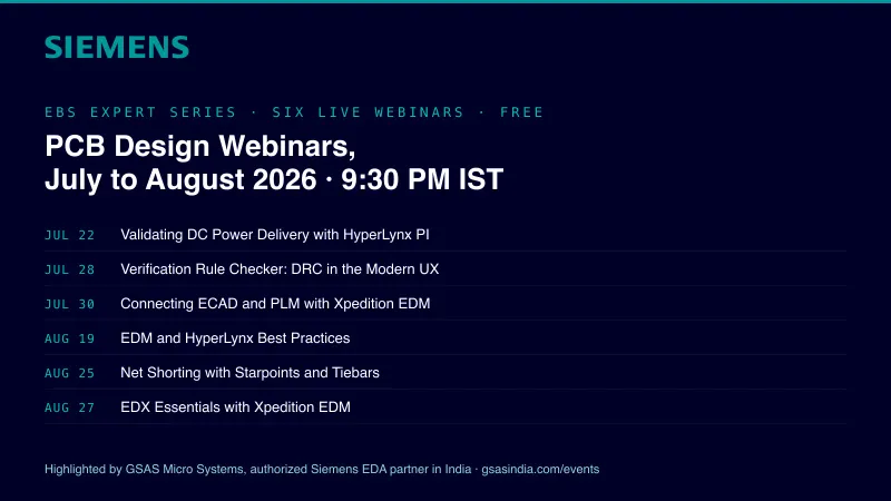
Siemens EDA EBS Expert Series: 6 Free PCB Design Webinars (Jul-Aug 2026)
20 Jul · 8 min
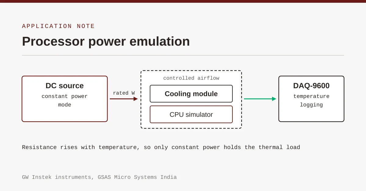
Emulating Processor Power for Thermal Testing: Why Constant Power
7 Oct · 7 min
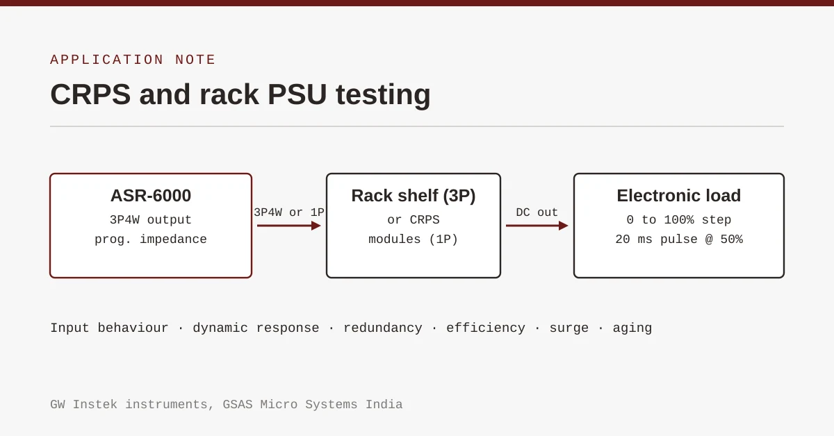
CRPS and Rack Power Supply Testing: The Six Tests That Matter
7 Oct · 7 min