In short
A solar array simulator is a programmable DC source that presents a photovoltaic I-V curve at its terminals instead of a stiff voltage, so a PV inverter's maximum power point tracking algorithm can be exercised indoors, on demand, and independent of weather, against curves that repeat exactly from one test run to the next.
A PV inverter is judged on how well it finds and holds the maximum power point of the array behind it, and that is hard to assess outdoors, because a real array never presents the same conditions twice. The instrument that solves it is a solar array simulator: a DC source programmed to behave like a photovoltaic array rather than like a power supply. This article covers what that means electrically, what static and dynamic MPPT testing ask of the inverter, and the specification detail that disqualifies otherwise suitable hardware.
What a Solar Array Simulator Is
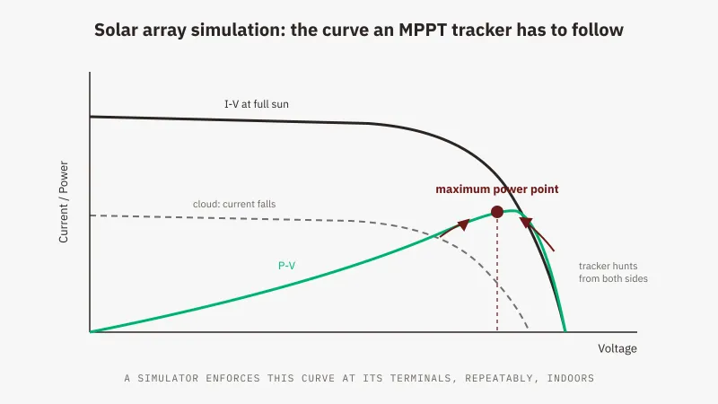
An ordinary bench supply is built to be stiff: set it to 400 V and it holds 400 V while the load draws whatever current it wants, up to the limit. A photovoltaic array behaves in the opposite way. Its terminals follow a curve: draw no current and you measure open-circuit voltage, short the terminals and you measure short-circuit current at zero volts, and every point in between sits on a characteristic set by the cell technology, the irradiance on the modules and the cell temperature.
A solar array simulator is a programmable DC source whose control loop enforces that curve at its output. It is still a power supply in the physical sense, but its setpoint is a shape rather than a number: pull more current and the terminal voltage collapses the way a real array’s would, back off and it recovers along the same path. Because the shape is programmed rather than observed it is repeatable, which is what turns array behaviour into a test fixture.
Why MPPT Testing Needs a Curve, Not a Supply
Power at any point on the curve is the product of voltage and current, and that product is zero at both ends: voltage without current at open circuit, current without voltage at short circuit. Between them it rises to a peak near the knee. That peak is the maximum power point, where the array delivers everything it has under the present conditions.
The peak does not stay put. Irradiance largely scales the current axis, so a passing cloud drags the curve down and the peak with it, while cell temperature largely moves the voltage axis, so the same array in the morning and in mid-afternoon presents different peaks under identical sunlight. An inverter therefore has to search continuously, and that search is the maximum power point tracking algorithm: in its simplest form it perturbs the operating point, observes whether power went up or down, and keeps moving in the direction that improves it.
A conventional supply cannot evaluate that. Feed the inverter from a stiff source and there is no curve to track, so power rises with current until the supply reaches its limit and the search converges on the instrument’s current limit rather than on any property of the inverter. Outdoor testing has the opposite problem: the curve is genuine but will not hold still and will not repeat, so two runs of the same firmware on the same roof are two different experiments and a regression cannot be attributed to the change under test.
Partial shading is where trackers fail in ways a clean curve never reveals. When part of a string is shaded, bypass diodes conduct around the affected substrings and the characteristic stops being one smooth hump. It develops several local maxima, one of which is the global peak and the rest of which are traps, and a hill-climbing algorithm that reaches a local one and finds no improvement in either direction can settle there and leave real energy unharvested. Presenting that shape deliberately requires a programmed curve.
Static and Dynamic MPPT Testing
Static MPPT testing holds one curve fixed. The questions are whether the algorithm finds the peak, how close to the available peak it settles, and how long it takes. Because the curve is programmed the peak is known, so extracted power is compared against available power directly rather than inferred. Repeat across curves covering low and high irradiance and cold and hot cells, since an algorithm well behaved at full sun behaves differently in the low-irradiance and cold-cell corners of the envelope.
Dynamic MPPT testing moves the curve while the inverter runs. Irradiance ramps test whether the tracker keeps up with a peak that is travelling, and irradiance steps test how it recovers when the peak jumps. Together they expose the central trade-off in any tracking algorithm: small, cautious perturbations settle tightly on a fixed curve but lag on a ramp, while larger, faster ones follow a moving peak but keep oscillating around it once conditions steady, spending energy on the search itself. Neither behaviour is visible on a static curve alone.
Cloud profiles are the realistic version of that stress, and cloud shading and cloud movement scenarios are documented capabilities of the Solar Array Simulation function on the GW Instek RBS Series, alongside static and dynamic MPPT testing. Cloud movement is the harder case, because on a real array a shadow crossing the strings is partial shading in motion: local maxima appear, shift and merge while the tracker is working, and the inverter has to decide when to abandon local hill-climbing and sweep the curve globally. Whether a given simulator scenario synthesises those multiple local maxima or ramps a single-knee curve is worth confirming before you rely on it, and where the firmware draws its re-sweep line is a behaviour worth measuring rather than assuming.
Profiles and Models: EN50530, Sandia, SAS2 and User-Defined
Taking the RBS Series as the worked example, GW Instek lists the curve sources as PV SAS, EN50530 and Sandia modes, plus SAS2 and user-defined models.
EN50530 is the European standard covering the overall efficiency of grid-connected photovoltaic inverters, including procedures for dynamic MPPT efficiency testing. Selecting it means the curves driving your test align with a recognised published method, which is what makes a tracking result comparable between laboratories rather than internal to yours. Work from the published standard for the procedure details.
Sandia refers to the photovoltaic array performance model published by Sandia National Laboratories, which derives array behaviour from module-level parameters. It suits work where the curve should follow from the modules you intend to deploy.
SAS2 and user-defined models are the remaining curve sources. GW Instek documents them by name; the parameter set each accepts is a question for the datasheet and the demo rather than this article, and the user-defined slot is where a stress curve built to break a particular algorithm would live.
The Voltage-Class Trap: SAS Is Not on Every Model
This is the detail that costs purchase orders. Solar Array Simulation is listed as a standard function on the RBS Series, and the footnote attached says models rated 500 V and above. The 100 V class does not carry it, GW Instek does not list it as an upgrade option, and no amount of parallel connection creates it.
That matters because the 100 V class is otherwise attractive: it carries the series’ largest single-unit currents and is the natural pick for low-voltage work. A team specifying one instrument for a mixed lab can land on it, read Solar Array Simulation on the family feature list, and find the footnote after delivery. If PV inverter testing is anywhere in scope, the whole 100 V class leaves the shortlist before any other criterion applies.
Once you are at 500 V or above, the string you intend to reproduce sets the class, and PV inverter work typically lands at 1000 V or 1500 V. One PV-specific sizing note: open-circuit voltage rises as cell temperature falls, so a string’s cold-morning maximum, not its nameplate operating voltage, is what the instrument has to clear. The rest of the selection sequence, including the model-number verification habit this footnote teaches, is in our guide to how to choose a regenerative bidirectional DC power supply.
Bench Design Notes
A solar array simulator replaces the array and nothing else. It sources the DC side, while the inverter’s AC output still has to go somewhere: a grid connection under a laboratory interface, or a load bank or grid simulator where a real connection is not available. Sizing the output side is a separate exercise, and a common first-layout omission.
On the RBS Series the simulator happens to be a bidirectional, regenerative instrument. That changes little during PV simulation itself, where power flows out into the inverter throughout, but it matters for what else the chassis does on other days, when battery or converter work sends energy back the other way, an architecture covered in how a regenerative bidirectional DC power supply works.
For string-level power beyond one chassis, up to ten identical units run in master-slave parallel, and a model’s system ceiling is ten times its own rating. Two consequences follow: parallel operation scales current and power rather than voltage (the only voltage stacking GW Instek documents is the 100 V class’s two-unit series option, capped at 300 V combined, which does not reach string territory), so the voltage class has to be right on its own, and parallelling low-voltage units does not add a function they lack.
Long dynamic MPPT profiles become unattended runs, so set the protection envelope before you start; the full protection suite is on the product page. The supplied PC control software covers PV mode along with data recording, which is where MPPT efficiency numbers come from once a run finishes.
Where GSAS Fits
GSAS Micro Systems is an engineering partner for GW Instek in India, and the useful part of our involvement in a PV test bench happens before the order is placed. We work through the string voltage and current envelope you need to reproduce, confirm that the model under consideration carries the Solar Array Simulation function rather than assuming the family list applies, and check your facility’s three-phase supply against the instrument’s input window.
Full ratings for the RBS Series 500 V and above models, SAS availability and India pricing are on the product page. We arrange demos and evaluation units, and support installation, calibration and after-sales from offices in Bengaluru, Hyderabad, Chennai, Pune, Mumbai and Delhi NCR.
Request a quote with the array curves you need to reproduce, and the reply will name the model, confirm Solar Array Simulation on it in writing, and flag the AC-side sizing alongside.
Also appears in:
Interested in GW Instek tools?
Talk to our application engineers for personalized tool recommendations.
More from GW Instek
View all →
Emulating Processor Power for Thermal Testing: Why Constant Power
7 Oct · 7 min
CRPS and Rack Power Supply Testing: The Six Tests That Matter
7 Oct · 7 min
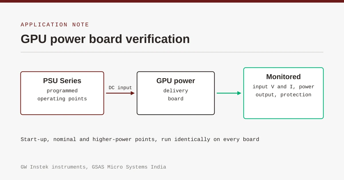
GPU Power Board Testing: DC Input Verification Before Integration
7 Oct · 6 min
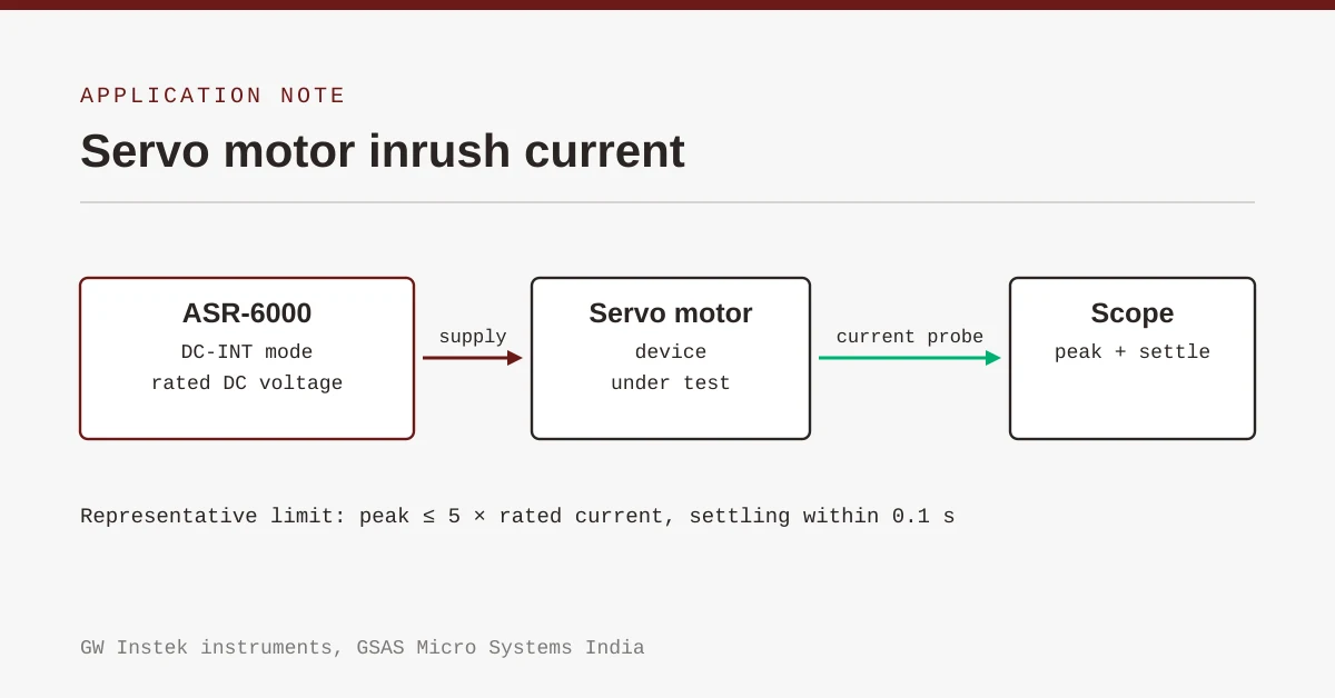
Servo Motor Inrush Current Testing: Method, Limits and Bench
7 Oct · 6 min
SuperTest Van Gogh 6.0: C23, C++23 and the C++20 Modules Gap
6 Oct · 7 min
AI Inside the Engineering Process: What Is Worth Automating, and What Still Needs an Engineer
21 Sept · 11 min