
The Battery Life Credibility Problem
Every IoT product datasheet includes a battery life claim. “Up to 5 years on 2xAA batteries.” “10-year coin cell operation.” These claims are central to the product’s value proposition, they determine whether the product is viable for the intended application. But how many of these claims are backed by rigorous measurement?
In many Indian IoT product companies, battery life claims are derived from spreadsheet calculations using datasheet typical values for component current consumption. The MCU datasheet says 1.2 uA sleep current. The radio datasheet says 8 mA for 2 ms per transmission. Multiply, divide, and the spreadsheet says 7.3 years. The number looks precise, but it is an estimate built on best-case assumptions.
The reality is that the actual sleep current is 3.5 uA (because of GPIO configuration, regulator quiescent current, and sensor leakage). The actual transmission event takes 12 ms (because of protocol overhead, retransmissions, and receive windows). The actual battery life is 2.1 years, less than a third of the claim.
Measurement-based battery life testing replaces assumptions with data. The Joulescope JS220 provides the measurement capability, nanoamp resolution, 2 Msps sampling, simultaneous current and voltage, to characterize every aspect of an IoT device’s power budget and produce battery life predictions with quantified confidence.
Phase 1: Duty Cycle Characterization
Capture the Complete Operating Cycle
Connect the Joulescope in series with the device’s power supply and capture multiple complete duty cycles. A duty cycle is one complete period from the start of one sleep phase to the start of the next, encompassing all active operations: wake-up, sensor read, data processing, radio transmission, receive window, and return to sleep.
For a device that wakes every 15 minutes, capture at least 20 cycles (5 hours of data). The Joulescope’s 2 Msps continuous sampling captures every transient within each cycle, and the unlimited capture duration handles the long sleep periods between cycles without dropping data.
Identify Every Operating State
Use the Joulescope UI’s oscilloscope view to zoom into individual duty cycles and identify each operating state by its current signature. Annotate each state with its duration and current magnitude. Common states that engineers miss in spreadsheet models:
- Oscillator settling time: Crystal oscillators take 0.5 to 5 ms to stabilize after wake-up, during which the MCU draws active current while waiting. RC oscillators start faster but are less accurate.
- Radio listen-before-talk: Some protocols require the device to listen for channel activity before transmitting, drawing receive current for a variable duration.
- Protocol acknowledgment windows: LoRaWAN requires two receive windows (RX1 and RX2) after each uplink. Even if the acknowledgment arrives in RX1, the device may still briefly power the radio for RX2.
- Sensor warm-up: Many sensors require a stabilization period after power-on. A gas sensor might need 10 seconds at milliamp-level current before its first valid reading.
Compute Energy Per Cycle
For each captured duty cycle, compute the total energy consumed:
Energy (joules) = integral of [V(t) x I(t)] dt over one complete cycle
The Joulescope UI computes this automatically. For scripted analysis, the Python API provides the raw data for numerical integration.
With 20+ cycles measured, compute the mean energy per cycle and the standard deviation. The standard deviation captures the real variability, variable radio transmit times, retransmissions, sensor conditioning differences, that no spreadsheet model can predict.
Phase 2: Sleep Current Deep Dive
Sleep current deserves separate, dedicated measurement because it dominates the battery life equation for duty-cycled devices. A device that wakes for 50 ms every 15 minutes spends 99.99% of its time in sleep. At that duty cycle, a 1 uA increase in sleep current consumes more energy than doubling the active-phase current.
Measure sleep current over a 60-second window with all peripherals in their production sleep state. Look for:
- Periodic micro-wakes: RTC tick interrupts, watchdog refresh cycles, or peripheral calibration events that briefly elevate current at regular intervals
- Parasitic leakage: Current that does not correspond to any firmware activity, typically caused by pull-up resistors on floating lines, reverse leakage through protection diodes, or sensor standby current
- Voltage regulator quiescent current: The regulator’s own current consumption, which is independent of load current and sets the floor for system sleep current
Phase 3: Battery Life Projection
Average Current Method
Average current = (energy per cycle / cycle period) / average voltage
For a device consuming 1.2 mJ per 15-minute cycle at 3.0 V average voltage:
Average current = 1.2 mJ / (900 s x 3.0 V) = 0.44 uA
Battery life = 2500 mAh (2xAA) / 0.00044 mA = approximately 5.7 million hours = approximately 648 years
That number is clearly unrealistic because it ignores battery self-discharge (which is typically 1-3% per year for alkaline cells and higher for lithium primaries at elevated temperatures). The practical battery life is limited by self-discharge, not device consumption, for ultra-low-power devices.
Realistic Projection
Include battery self-discharge current (typically 2-10 uA equivalent for AA alkaline cells) in the average current calculation. Also account for battery voltage decay, as the battery discharges, the terminal voltage drops, which may cause the voltage regulator to enter dropout, increasing its quiescent current and potentially causing the device to reset and re-initialize (consuming more energy per cycle).
The Joulescope’s simultaneous voltage measurement captures the actual supply voltage during each duty cycle, enabling the engineer to identify the minimum operating voltage and calculate the usable battery capacity (which is less than the rated capacity when the cutoff voltage is above the battery’s end-of-life voltage).
Phase 4: Accelerated Validation
Validate the projection with an accelerated test. Increase the duty cycle frequency, if the device normally wakes every 15 minutes, configure it to wake every 15 seconds (a 60x acceleration). Run the accelerated test for 24 to 48 hours while continuously logging energy with the Joulescope.
Compare the measured cumulative energy against the projection. If they agree within 5%, the projection is validated. If they diverge, investigate temperature effects, battery voltage decay, and time-dependent leakage.
Why Buy Joulescope From GSAS
GSAS provides Joulescope instruments with INR invoicing and application support from offices in Bengaluru, Hyderabad, Chennai, Pune, Mumbai, and Delhi NCR. Our team supports IoT product teams building measurement-based battery life validation into their development process.
Contact sales@gsasindia.com or call +91 80 6590 1783.
Also appears in:
Interested in Joulescope tools?
Talk to our application engineers for personalized tool recommendations.
More from Joulescope
View all →
Battery Discharge Profiling for Coin Cell Devices: From CR2032 to 10-Year Life
5 Apr · 7 min
BLE Power Profiling: Measuring Bluetooth Low Energy Current With Joulescope
5 Apr · 7 min
Energy Harvesting and Power Measurement: Designing Self-Powered IoT Devices
5 Apr · 7 min

IoT Power Consumption Trends: Why Indian Product Teams Need Better Measurement
5 Apr · 7 min
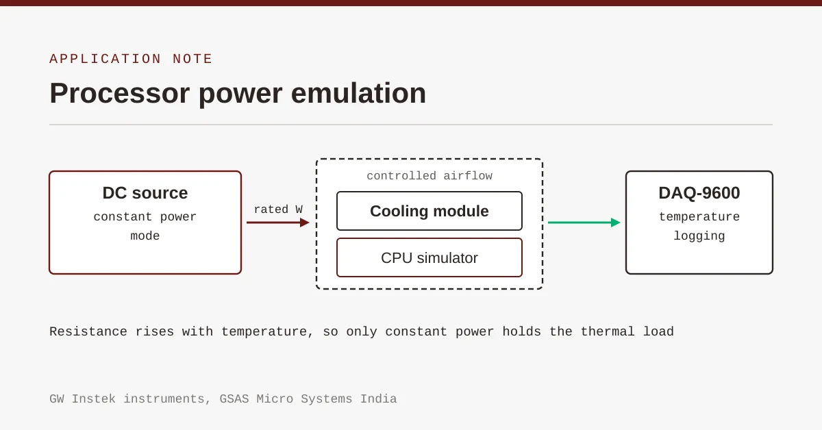
Emulating Processor Power for Thermal Testing: Why Constant Power
7 Oct · 7 min
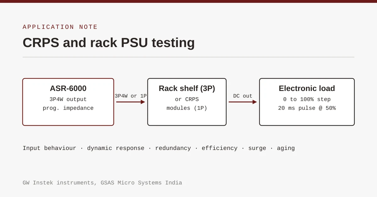
CRPS and Rack Power Supply Testing: The Six Tests That Matter
7 Oct · 7 min