In short
ADAS sensor data logging captures raw or compressed camera, radar and lidar streams in a test vehicle alongside bus traffic. Budget it by multiplying horizontal pixels by vertical pixels by frame rate by bits per pixel for each camera, points per second by bytes per point for each lidar, and receive channels by samples by chirps by frame rate by bytes per sample for each radar, then divide by 8 for bytes per second and multiply by 3,600 for bytes per hour. A 1920 by 1080 camera at 30 frames per second and 12 bits per pixel is 746.496 Mbit/s, which is 93.312 MB/s, which is 335.92 GB per hour. Match the capture point, the logger uplink and the sustained media write rate to the total, not to the link rate.
Search for how much data an ADAS test vehicle produces and you get headline numbers: terabytes per day, tens of gigabits per second, a storage figure with a plus sign after it. What you almost never get is the arithmetic behind the headline, so you cannot check it and cannot redo it for the sensor set going into your vehicle next month.
This article is the arithmetic. One formula, worked once in full, and a table where every row is derived on the page from it, so you can substitute your own resolution, frame rate and bit depth. Then the two consequences nobody carries through: where the capture point has to sit, and whether the storage sustains the write rate for the whole drive.
Rule for this page. Any number not derived here is attributed to a named source, listed in full at the end. Decimal units throughout, the same convention as our data logger article: 1 MB is 10 to the power 6 bytes, 1 GB is 10 to the power 9, 1 TB is 10 to the power 12, which is how media is sold and how link rates are quoted.
What an ADAS logging session actually has to capture
Sensor streams and bus traffic are two different problems
Sensor streams are wide and continuous: a camera emits the same bits every frame whether anything happened or not. Bus traffic is narrow and bursty: a CAN frame tells you what a controller decided. Bandwidth belongs almost entirely to the first. Meaning belongs largely to the second.
Why they are logged together, and what that constrains
A perception defect is rarely visible in either stream alone. It is a camera frame, a radar object list and an actuation message disagreeing, and only one timeline shows that. Recording them together forces a single time base across sources with wildly different rates, and every stream through the same aggregation point and storage. The narrow streams cost almost nothing to carry, and are why the wide ones are worth keeping.
Raw sensor data versus perception output
The same sensor can be logged raw, as pixels, point clouds or radar ADC samples; as detections and object lists; or as fused perception output. Volume drops by orders of magnitude at each step, and so does what you can re-run offline, because an object list cannot be fed back through a detector under test. That is a validation decision before it is a storage one.
The bandwidth formula, written out
Worked once in full
For any camera stream:
horizontal pixels x vertical pixels x frames per second x bits per pixel = bits per second
For a 1920 by 1080 imager at 30 frames per second and 12 bits per pixel:
- 1920 x 1080 = 2,073,600 pixels per frame.
- 2,073,600 x 12 = 24,883,200 bits per frame.
- 24,883,200 x 30 = 746,496,000 bits per second, which is 746.496 Mbit/s.
Converting to bytes, and to volume
- Divide by 8 bits per byte: 93,312,000 bytes per second, which is 93.312 MB/s.
- Multiply by 3,600 seconds in an hour: 335,923,200,000 bytes, which is 335.92 GB per hour.
Every term is linear. Double the frame rate and the answer doubles; four times the pixels and it quadruples. The bits per pixel term is the stored depth, not the imager’s advertised depth, so a raw 12-bit Bayer frame, a 16-bit YUV422 frame and a 24-bit RGB frame from the same sensor give three different answers, all correct for their own container.
Where the formula understates reality
Four things sit on top of the result, and all four push it up.
Blanking. The formula counts active pixels. A link carries horizontal and vertical blanking intervals as well, so the wire rate exceeds the active pixel rate.
Per-frame metadata. Imagers emit embedded metadata lines carrying exposure, gain and frame counters, which are pixels on the link and bytes in the file.
Container overhead. Every stored frame carries a header, and the file carries an index. Small per frame, thousands of frames per minute.
Packetisation. On a network, each packet carries link, network and transport headers, preamble and interframe gap on the wire, and any capture encapsulation header added on the capture path. That cost is per packet, not per byte, so it grows with fragmentation rather than with volume.
No percentages are offered here, because they depend on your container, encapsulation and packet size. Measure yours the way you would measure encapsulation overhead on a bus: capture a known number of frames, divide file size by frame count, use that. Until then, treat the formula’s answer as a floor.
Per-sensor bandwidth table
Every row is derived from a stated configuration using the formula above. Substitute your own numbers into the derivation column and the arithmetic is the same. Decimal units, GB per hour.
| Sensor and stated configuration | Derivation | Raw rate | Raw GB/hour |
|---|---|---|---|
| Camera, 1280 x 800, 30 fps, 12 bpp | 1,024,000 x 12 x 30 | 368.64 Mbit/s (46.08 MB/s) | 165.89 |
| Camera, 1920 x 1080, 30 fps, 12 bpp | 2,073,600 x 12 x 30 | 746.496 Mbit/s (93.312 MB/s) | 335.92 |
| Camera, 1920 x 1080, 30 fps, 16 bpp | 2,073,600 x 16 x 30 | 995.328 Mbit/s (124.416 MB/s) | 447.90 |
| Camera, 3840 x 2160, 30 fps, 12 bpp | 8,294,400 x 12 x 30 | 2.985984 Gbit/s (373.248 MB/s) | 1,343.69 |
| Camera, 3840 x 2160, 60 fps, 12 bpp | 8,294,400 x 12 x 60 | 5.971968 Gbit/s (746.496 MB/s) | 2,687.39 |
| Lidar, 64 ch x 1,024 columns x 10 rev/s, one return, 16 B/point | 655,360 points/s x 16 | 83.886 Mbit/s (10.486 MB/s) | 37.75 |
| Lidar, 10.4 M points/s, 16 B/point | 10,400,000 x 16 | 1.3312 Gbit/s (166.4 MB/s) | 599.04 |
| Lidar, 10.4 M points/s, 8 B/point | 10,400,000 x 8 | 665.6 Mbit/s (83.2 MB/s) | 299.52 |
| Imaging radar, raw cube: 16 RX x 512 samples x 256 chirps x 20 fps, 4 B/complex sample | 41,943,040 samples/s x 4 | 1.342 Gbit/s (167.77 MB/s) | 603.98 |
| Imaging radar, object list: 256 objects x 32 B x 20 fps | 163,840 B/s | 1.311 Mbit/s (0.164 MB/s) | 0.59 |
| Ultrasonic, 12 sensors x 40 readings/s x 16 B | 7,680 B/s | 0.061 Mbit/s (0.0077 MB/s) | 0.028 |
| GNSS and IMU, 200 Hz x 9 channels x 4 B, plus 10 Hz x 100 B | 8,200 B/s | 0.066 Mbit/s (0.0082 MB/s) | 0.030 |
| 100BASE-T1 link, both directions at ceiling | 2 x 100 Mbit/s | 200 Mbit/s (25 MB/s) | 90.00 |
| 1000BASE-T1 link, both directions at ceiling | 2 x 1,000 Mbit/s | 2 Gbit/s (250 MB/s) | 900.00 |
| CAN at 500 kbit/s, fully loaded | 500,000 / 8 | 500 kbit/s (0.0625 MB/s) | 0.225 |
Two rows need their configuration explained.
The high lidar row. A public lidar product page states 128 channels of vertical resolution and 10.4 million points per second. Channels multiplied by columns per revolution, by revolutions per second, by returns is what lands there, and the vendor does not publish which combination it used, so take the points-per-second figure and set the bytes per point yourself. A Cartesian point stored as x, y, z and intensity in four 32-bit fields is 16 bytes, and a compact native range and reflectivity encoding is nearer 8. Both rows are shown so the factor of two your storage format costs you is visible. A 10.4 million point per second lidar at 16 bytes per point is 1,331.2 Mbit/s (166.4 MB/s), and at 8 bytes per point it is 665.6 Mbit/s (83.2 MB/s).
The radar rows. Raw ADC data and object lists differ by about a factor of 1,000 on the same sensor, which is why “radar data rate” means nothing without saying which one. Substitute your receive channel count, chirp parameters and frame rate.
The bus rows are link ceilings, not offered load. IEEE 802.3bw Clause 96 specifies 100BASE-T1 as 100 Mbit/s full duplex over a single balanced pair, and IEEE 802.3bp Clause 97 specifies 1000BASE-T1 as 1 Gbit/s the same way; our T1 family guide traces both to the task force documents. Capturing a full duplex link means capturing both directions, hence the doubling. A link that can carry 1 Gbit/s rarely does, so budgeting on the ceiling oversizes the logger and budgeting on last week’s average undersizes it. Measure offered load on your own network, then add margin.
The encoded column
There is no honest single compression ratio for this table, and that is a fact about encoders rather than a gap in the research: they are rate controlled, so the output bit rate is a parameter you set and the quality falls out. The only ratio relationship a standards body publishes is between codecs, not against raw. ITU stated on 25 January 2013 that HEVC, standardised as ITU-T Recommendation H.265, “will need only half the bit rate of its predecessor”, H.264, so at equal perceptual quality the move from H.264 to H.265 roughly doubles whatever ratio you were getting.
The encoded column is therefore a bit rate you choose, with the ratio derived from it:
| Encode bit rate | MB/s | GB/hour | Ratio against 1920 x 1080 raw | Ratio against 3840 x 2160 raw |
|---|---|---|---|---|
| 10 Mbit/s | 1.25 | 4.50 | 74.6 to 1 | 298.6 to 1 |
| 25 Mbit/s | 3.125 | 11.25 | 29.9 to 1 | 119.4 to 1 |
| 50 Mbit/s | 6.25 | 22.50 | 14.9 to 1 | 59.7 to 1 |
| 100 Mbit/s | 12.5 | 45.00 | 7.5 to 1 | 29.9 to 1 |
Anyone quoting you a fixed compression ratio for automotive video is quoting their own encoder settings. Ask what bit rate, what codec, what profile, and what the quality target was.
Raw versus compressed: what the decision costs you
What lossy encode removes from a perception regression test
An encoder discards what a human viewer is unlikely to notice, and a detector is not a human viewer. The low-contrast edges, small distant objects and high-frequency texture that decide a marginal detection are what a rate-controlled encoder spends fewest bits on. Re-running a detector against an encoded log tests it against the encoder, not the road.
Lossless and visually lossless, and the honest limits
Lossless encoding reconstructs every original sample, so the evidence question disappears, but the ratios are far lower and vary with scene content rather than with a bit rate you set, which makes the budget harder to predict. Visually lossless means a viewer cannot tell, a claim about human perception and not about a detector. If the log is evidence for a perception decision, visually lossless is not lossless.
Encode latency and whether the log still reflects sensor timing
An encoder adds delay, and if the timestamp written into the file is applied after encoding rather than at capture, every timing conclusion inherits that delay. Timestamp at the capture point, carry it through the encode, and confirm the logger does not restamp.
The common hybrid
Raw for the sensor under investigation, encoded for the surrounding context. It works as long as one thing is written down: which streams were encoded, with what codec and settings. An undocumented encode discovered six months later invalidates the analysis built on it.
Where the capture point has to sit
SerDes links are not Ethernet
Uncompressed camera video runs over serialiser links, not over the network, so there is nothing for a packet capture tool to see. Our SerDes camera links article covers the families, rate classes and the record, replay and inject workflow in full. For a bandwidth budget the point is that the raw camera rows above are a sizing bound at the sensor, and a capture point on the Ethernet side sees something different. MIPI publishes A-PHY downlink gears of 2, 4, 8, 12 and 16 Gbit/s in v1.0 and v1.1, roughly what the raw camera rows demand.
Ethernet camera streams
Where video is placed on the vehicle network it is captured as network traffic, with the packetisation overhead noted above and the same tap or mirror decision as any other segment. Budget the encoded rates here, not the raw ones.
In-ECU logging, in-line tap, switch mirror
In-ECU logging is cheap and proves what the ECU believed. An in-line tap proves what was on the wire. A switch mirror proves what the switch chose to forward, and drops silently when the destination port is oversubscribed. Choose by what the recording has to prove.
The aggregation point
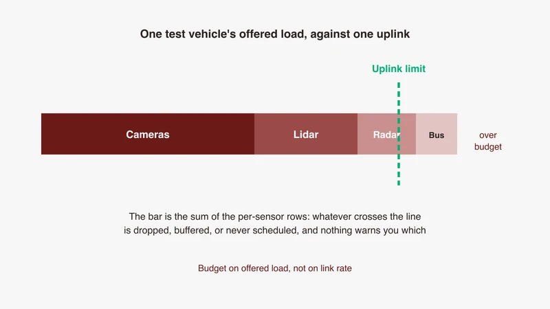
Every stream eventually meets one logger uplink, and that uplink is where budgets break. Sum the offered load across every capture point in bits per second and compare it with the uplink rate. If the sum exceeds the uplink, nothing downstream rescues it.
Storage throughput, not just storage capacity
Sustained write rate is the constraint
Datasheets quote burst and cache-assisted figures alongside a sustained sequential write rate, and only the last describes an eight-hour drive. Ask for sustained sequential write with the cache exhausted, how it degrades as the media fills, and at the temperature the media will see.
Capacity sizing from the table
Capacity is the easy half: sensors x hours x GB per hour, straight from the table. It is easy enough that programmes size for it and lose frames anyway, because the drive was big enough and the write path was not fast enough.
Removable media, offload and the ingest bottleneck
Offload has to fit in the gap between shifts, and the lab then has to ingest, index and back up what arrives, a data-management problem our telematics unit deep dive picks up at fleet scale. That side of the chain is routinely left out of the budget, and is routinely what limits how many test days a week a programme can run.
Vibration, temperature and power
Vibration, a wide temperature range and an unclean supply narrow the media choice, and thermal throttling turns a datasheet write rate into a lower real one halfway through a summer drive in Pune. Size for the throttled rate.
Worked example: an eight hour test drive
The sensor set
Four cameras at 1920 by 1080, 30 fps, 12 bpp, raw. One camera at 3840 by 2160, 30 fps, 12 bpp, raw. One lidar at 10.4 million points per second, 16 bytes per point. Four imaging radars streaming object lists. Twelve ultrasonic sensors. GNSS and IMU. Two 1000BASE-T1 backbone links captured in both directions at 30 percent offered load. Four CAN buses at 500 kbit/s and 40 percent load.
Row by row
| Line | Derivation | MB/s |
|---|---|---|
| 4 x 1920 x 1080 cameras | 4 x 93.312 | 373.248 |
| 1 x 3840 x 2160 camera | 1 x 373.248 | 373.248 |
| Lidar | 10,400,000 x 16 | 166.400 |
| 4 x radar object lists | 4 x 0.16384 | 0.655 |
| Ultrasonic | 12 x 40 x 16 | 0.008 |
| GNSS and IMU | 7,200 + 1,000 B/s | 0.008 |
| 2 gigabit links, both directions, 30 percent | 2 x 2 x 1,000 x 0.30 Mbit/s | 150.000 |
| 4 CAN at 40 percent | 4 x 500 x 0.40 kbit/s | 0.100 |
| Total | 1,063.67 |
Total rate, volume, offload window, media count
- Sustained aggregate: 1,063.67 MB/s, which is 8,509.3 Mbit/s, or 8.51 Gbit/s.
- Per hour: 1,063.67 x 3,600 = 3,829.20 GB.
- Eight-hour shift: 3,829.20 x 8 = 30,633.6 GB, which is 30.63 TB.
- Media at 8 TB per removable drive: 30.63 / 8 = 3.83, so four drives per shift, and the count is per shift, not per week.
- Offload over a 10 Gbit/s wired path achieving 8 Gbit/s in practice, which is 1 GB/s: 30,633.6 seconds, which is 8.51 hours. Over a 1 Gbit/s path achieving 100 MB/s it is 85 hours.
Read point 5 again. Offloading this drive takes longer than driving it, which decides how many vehicles a programme can run against one ingest bay and never appears in a bandwidth headline. Note also that 8.51 Gbit/s leaves a 10 Gbit/s logger uplink at 85 percent utilisation on the average, with no burst headroom, so this set needs the load split across more than one uplink.
The same set with encode applied
Encode all five camera streams at 50 Mbit/s each. That replaces 746.496 MB/s with 5 x 6.25 = 31.25 MB/s, a ratio of 23.9 to 1 against raw.
- New aggregate: 1,063.67 minus 746.496 plus 31.25 = 348.42 MB/s, which is 2.79 Gbit/s.
- Per hour: 1,254.32 GB. Eight-hour shift: 10.03 TB.
- Media at 8 TB: two drives. Offload at 1 GB/s: 10,034 seconds, under three hours.
All three constraints move together, and one thing changes character. Lidar is now 166.4 of 348.42 MB/s, 47.8 percent of the entire budget, and unlike the cameras there is no point-cloud codec sitting in the logging pipeline as a matter of course, so that 47.8 percent does not have an encoder to hand it to. Encode the cameras and your storage problem becomes a lidar problem.
What changes if one camera goes from 2 MP to 8 MP
Swap one 1920 by 1080 stream for a 3840 by 2160 stream and the raw budget rises by 373.248 minus 93.312, which is 279.936 MB/s. Over eight hours that is 8,062.2 GB, or 8.06 TB added to a single shift by one camera, taking the total to 38.70 TB and the media count to five drives. One line in a sensor specification, one extra drive to carry, and roughly two and a quarter extra hours of offload, taking the window from 8.51 hours to 10.75 hours.
Timestamps and metadata that make the volume useful later
One time base across sensors and buses
Thirty terabytes with an untrustworthy timeline is thirty terabytes of anecdote. Sensor and bus streams have to land on one time base, which in practice means a synchronised network clock and timestamps applied at the capture point. Our multi-bus capture article covers correlation across bus types, and gPTP troubleshooting covers what has to work before any of it holds. Validating the synchronisation itself is a separate exercise, and it belongs before the drive.
Session metadata to record at capture time
Sensor configuration for every stream, because the arithmetic above cannot be rechecked without it. Database and description files by version. Firmware and software versions. Which streams were encoded and with what settings. Route, driver, weather and time. Clock source, and whether the synchronised flag was set.
Indexing and trigger-based extraction
A 30 TB day that can only be read sequentially is not searchable. Build the index during capture, mark events during the drive with a physical marker input, and define trigger conditions in advance so windows can be extracted without a full pass. Bus-level decode alongside the sensor streams is what makes those triggers meaningful, which is where instrument-level bus decode and logger triggers meet.
Five ways bandwidth budgets go wrong
1. Budgeting on link rate rather than offered load
A gigabit link in the budget becomes 900 GB per hour in the sizing while the segment carries a fifth of that. The reverse error is worse: sizing to a measured average from a quiet bench, then meeting the real load on the road.
2. Budgeting on average rather than sustained peak
Sensors burst too, because a frame arrives during the active interval and the link idles through blanking, and buses and event-driven streams burst on top of that. The moment the vehicle does something interesting is the moment the peak arrives. A path sized to the average drops frames exactly when the recording matters.
3. Forgetting the return path and control traffic
Full duplex means two directions, and capturing a link means capturing both. Diagnostic sessions, camera control back channels, time synchronisation messages and logger management traffic all consume budget no per-sensor table lists.
4. Ignoring the offload and ingest side
The worked example took 8.51 hours to offload an eight-hour drive. Programmes plan the in-vehicle chain in detail and discover the lab chain in week three.
5. Treating an encoded log as equivalent evidence to a raw one
The cheapest way to make a budget work is to encode everything, and it is cheap because it quietly changes what the recording can prove. That is a validation decision, and it belongs to the people who own the validation plan, in writing, per stream.
What the published headline figures actually mean
Three widely cited aggregate figures are worth putting through the formula, since that is the whole point of this page.
Eurotech, writing about ADAS engineering challenges, states that total ADAS sensor bandwidth “can reach 40Gbit/s” and that “in less than 8 hours, when stored in raw format, this data would require over 127TB storage”. That reconciles: 40 Gbit/s is 5 GB/s, which is 18 TB per hour, and 127 divided by 18 is 7.1 hours.
Premio, writing about recording raw ADAS data on test drives, cites an Intel estimate of “4TB of data per vehicle per day”. Through the formula, 4 TB over an eight-hour day is 138.9 MB/s, or 1.11 Gbit/s: about one and a half raw 1920 by 1080 camera streams. Over 24 hours it is 370 Mbit/s. A figure that sounds enormous is a modest sensor set once divided by time.
Lexar Enterprise, writing on ADAS memory requirements, states “1.5-3 Gbps of raw image data per camera stream” and, on the same page, that a “6-camera + 4-ultrasonic + 2-radar configuration generates approximately 40+ GB of raw sensor data per hour”. The per-camera figure is reproducible: a 2560 by 1440 imager at 30 fps and 16 bpp is 1.769 Gbit/s by the formula, inside the stated range. The aggregate is not consistent with it. Six streams at 1.5 Gbit/s is 9 Gbit/s, which is 4,050 GB per hour, about a hundred times the stated aggregate. Both cannot describe the same configuration, and there is no arithmetic on the page to say which to use.
That is the case for deriving your own rows. Not because published figures are careless, but because a number without its derivation cannot be checked, adapted, or defended in a design review.
Where GSAS fits
GSAS Micro Systems is an engineering partner, and on ADAS logging the useful conversation happens before anything is specified. The arithmetic on this page is the conversation: your sensor list, resolutions and frame rates, lidar and radar configurations and bus load, run through the same formula until there is a sustained aggregate rate, a per-shift volume, a media count and an offload window your programme can live with.
Three decisions follow from those numbers rather than preceding them. Where the capture point sits for each stream, which is a different answer for a serialiser camera link than for a backbone segment. Whether one logger uplink carries the total or the load has to be split. And what the storage has to sustain, at temperature, with the cache exhausted, for the whole shift. Our applications engineers work in IST, so a working session lands inside your day, and the teams we work with sit in Bengaluru, Pune, Chennai, Hyderabad, Mumbai and Delhi NCR.
Start with the automotive Ethernet capability page, then request a scoped conversation with your sensor list and how long you need to record. If your existing setup already meets the budget once the arithmetic is done, that is a perfectly good outcome and you will hear it from us.
References
- IEEE 802.3 Ethernet Working Group: https://www.ieee802.org/3/
- IEEE P802.3bw D1.2 approved working group ballot comments (Clause 96, 100BASE-T1 at 100 Mbit/s full duplex over a single balanced twisted pair): https://www.ieee802.org/3/bw/comments/8023bw_D1_2_approved.pdf
- IEEE P802.3bp D1.4 Clause 97 draft text (1000BASE-T1 at 1 Gbit/s full duplex over a single balanced pair, PAM3 at 750 MBd): https://www.ieee802.org/3/bp/public/may15/tu_3bp_02a_0515.pdf
- MIPI Alliance, A-PHY specification page (downlink gears of 2, 4, 8, 12 and 16 Gbit/s in v1.0 and v1.1; up to 15 m reach): https://www.mipi.org/specifications/a-phy
- ITU-T Recommendation H.264, “Advanced video coding for generic audiovisual services”: https://www.itu.int/rec/T-REC-H.264
- ITU-T Recommendation H.265, “High efficiency video coding”: https://www.itu.int/rec/T-REC-H.265
- ITU press release, “New video codec to ease pressure on global networks”, Geneva, 25 January 2013 (HEVC “will need only half the bit rate of its predecessor”): https://www.itu.int/net/pressoffice/press_releases/2013/01.aspx
- Lidar manufacturer public product page (128 channels of vertical resolution; 10.4 million points per second), used only for the stated lidar configuration that the table row is derived from: https://ouster.com/products/hardware/os1-lidar-sensor
- Eurotech, “ADAS: solving the challenges” (aggregate context only: total ADAS sensor bandwidth can reach 40 Gbit/s; over 127 TB in less than 8 hours stored raw): https://www.eurotech.com/blog/adas-solving-the-challenges/
- Premio, “Computers to record raw ADAS sensor data during test drives” (aggregate context only: Intel estimate of 4 TB per vehicle per day): https://premioinc.com/blogs/blog/computers-to-record-raw-adas-sensor-data-during-test-drives
- Lexar Enterprise, “ADAS and memory requirements” (aggregate context only: 1.5 to 3 Gbit/s per raw camera stream; 100 to 200 MB/s lidar point cloud; 10 to 100 MB/s radar; approximately 40+ GB per hour for a stated 6-camera configuration): https://lexarenterprise.com/adas-and-memory-requirements/
Also appears in:
Building for Automotive & Mobility?
Talk to our application engineers for personalized tool recommendations.