In short
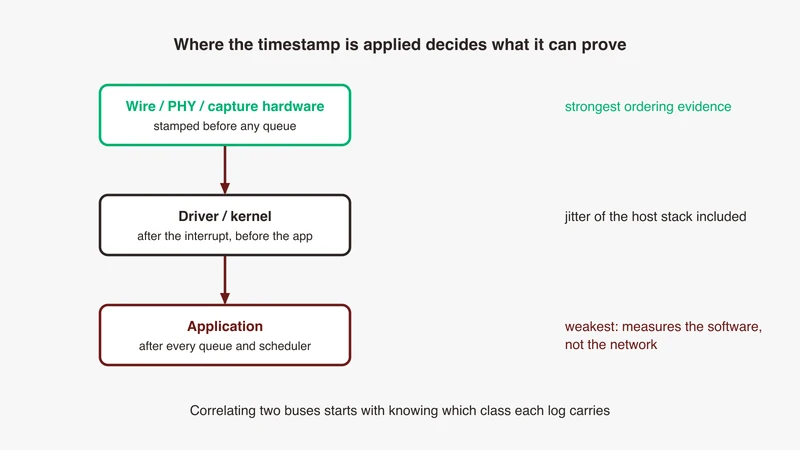
Correlating CAN, LIN, FlexRay and Ethernet means putting every frame on one time base rather than merging logs from independently clocked tools. Capture all buses through hardware-timestamped modules disciplined by a shared clock, then align. Where the timestamp is applied decides what it can prove: an application-level timestamp carries the host operating system's scheduling jitter, a kernel socket timestamp is taken just after the driver hands the packet to the receive stack, and a hardware timestamp is generated by the adapter itself. Only the hardware class, on a disciplined clock, supports an ordering claim between two buses.
Two logs of the same test. The CAN log has the request going out at 12.483. The Ethernet capture has the response arriving at 12.461. The answer preceded the question, which did not happen, and the session is now guesswork.
This is the most repeated complaint in vehicle network forum threads, and the answers are thin. Product pages assert their own synchronisation without explaining the mechanism; forum replies stop at “use one tool for everything”, advice about procurement rather than about time.
The mechanism is not complicated. Every frame gets a timestamp somewhere between the wire and your file, where it is stamped decides what the number can prove, and unless both buses were stamped against one clock, no post-processing makes two files one timeline. Proving the shared clock itself is the subject of validating time sync.
Why two logs of the same event do not line up
Independent clocks, independent start moments, independent drift
Two instruments produce three independent error terms, and treating them as one is where most attempted fixes fail.
Offset. The tools started their clocks at different moments. Constant, and the only term one alignment marker removes.
Drift. Their oscillators do not run at the same rate, so the gap widens as the session runs. The design house overview of timestamping in multi-ECU systems cited in our capture methods guide gives a typical crystal drift of 20 to 50 parts per million, or 20 to 50 microseconds of error per second. At the low end a two-hour soak accumulates 0.144 seconds, so an alignment done at minute zero is worth nothing at minute one hundred and twenty.
Jitter. Each capture path adds random variation. It does not accumulate the way drift does, and it does not cancel either, because you are making one measurement rather than averaging many.
Where the timestamp is actually applied: application, driver, or capture hardware
“The timestamp” is not one thing. A frame crosses the PHY, the adapter, the driver, the kernel receive stack and finally your capture application, and each height at which it can be stamped adds everything below it to the error.
The error budget: offset you can correct for, jitter you cannot
Offset comes out with one shared anchor event. Drift comes out with two, start and end, because two points define a linear correction. Jitter does not come out at all: it is the floor, and the floor decides whether your conclusion is measurement or opinion.
Why “close enough” fails exactly when the question is causality
Twenty microseconds of uncertainty is irrelevant when the question is “did this message appear” and fatal when it is “which came first”. Causality turns on the sign of a difference, and the sign of a difference smaller than your jitter floor is noise. Gateway latency and whether the ECU or the network is late are both causality questions.
The gateway blame problem
Symptom observed on Ethernet, cause on CAN or LIN, gateway in between
Vehicle Service Pros, writing on network communications in modern vehicles in October 2025, puts the gateway’s job plainly: gateway modules were introduced to allow messages travelling on different networks to be shared. Its example is vehicle speed arriving on CAN from the engine and translated to LIN for interior controls, so the doors lock at a programmed speed threshold.
So the argument starts like this. A service call goes out on Ethernet, the gateway translates it to CAN, an ECU responds, and the gateway translates back. Somebody watching only Ethernet reports responses 40 ms late; the ECU’s supplier replies that it responded in 6 ms. Both can be true.
Why an uncorrelated trace pair cannot distinguish a slow gateway from a late source
The Ethernet trace gives you one interval: request out, response in. Inside it sit three delays, gateway forward, ECU turnaround and gateway return: one observation, three unknowns. An uncorrelated CAN trace helps less than it feels like it should: it gives the ECU turnaround in the CAN log’s own time, but cannot place that interval inside the Ethernet one, because the two rulers have an unknown offset and drift between them.
What the trace has to show to assign blame: ingress time, egress time, one ruler
Four timestamps, one ruler: t1, request observed on Ethernet; t2, translated request observed on CAN; t3, response observed on CAN; t4, response back on Ethernet. Gateway forward latency is t2 minus t1, ECU turnaround is t3 minus t2, gateway return latency is t4 minus t3. The three add up to the interval the Ethernet-only view showed, and each now has an owner.
The same pattern in reverse for zonal architectures
Zonal designs move the problem rather than removing it. Traffic once observable on a vehicle-length bus now terminates a metre from the device that produced it, so a backbone capture shows what central compute saw rather than what the sensor sent, and the zone controller has taken over the gateway’s role, a shift our domain versus zonal comparison covers in full. The four-timestamp requirement is unchanged; the capture points move inside the zone. Our comparison of Ethernet and CAN covers why both survive.
Three classes of timestamp
Software timestamps taken in the host application
The application asks the operating system for the time when it receives a frame. The design house overview cited above is direct about the cost: capture in application software, after the frame has crossed the OS network stack, includes the scheduling jitter and interrupt latency the OS introduced, typically tens to hundreds of microseconds of variability.
Kernel or driver timestamps: better, still after the interface
The level most engineers are on without knowing. The Linux kernel documents SO_TIMESTAMP as generating a timestamp for each incoming packet in system time, described as not necessarily monotonic, and SO_TIMESTAMPING as generating timestamps on reception, transmission or both, from multiple sources including hardware. The flag wording matters. SOF_TIMESTAMPING_RX_SOFTWARE timestamps are generated, in the documentation’s words, just after a device driver hands a packet to the kernel receive stack. SOF_TIMESTAMPING_TX_SOFTWARE timestamps are generated in the device driver as close as possible to, but always prior to, passing the packet to the network interface, and require driver support that may not be present. Even the kernel timestamp therefore lands after the driver has handled the frame: it removes the application’s scheduling jitter, not the interface’s.
The CAN side is worth stating as documented rather than by analogy. SocketCAN’s documentation describes obtaining an accurate timestamp with an ioctl call after reading a message from the socket, with a resolution of one microsecond, set automatically at the reception of a CAN frame. That is a resolution statement, not an accuracy statement, and the kernel’s timestamping page does not discuss CAN. For a defensible CAN timestamp, go to the capture hardware.
Hardware timestamps applied at the capture interface or PHY
SOF_TIMESTAMPING_RX_HARDWARE and SOF_TIMESTAMPING_TX_HARDWARE request timestamps generated by the network adapter itself. This is the class that supports ordering claims, because the stamp lands before anything software-scheduled touches the frame.
The catch bites hardest here: hardware timestamps are not in your system clock’s time base. The kernel documentation deprecates its legacy field for hardware timestamps converted to system time, and says the intended approach is to expose the hardware clock on the NIC directly as a hardware PTP clock source, allowing conversion in userspace. A hardware timestamp is therefore precise against a clock you have not yet related to anything, and disciplining it is a separate job.
How to find out which class your setup is actually using
- On a Linux host,
ethtool -T <iface>reports timestamping capabilities and the PTP Hardware Clock index. No real PHC index means no hardware timestamps, whatever the tool’s configuration screen implies. - On an encapsulated capture, filter on the synchronisation flag the format carries. Frames flagged unsynchronised carry timestamps you may not quote.
- On any capture, run the two-anchor test below on a session you trust. Drift in the tens of microseconds per second means a free-running clock.
Timestamp source versus what it can prove
Accuracy below is a class, not a datasheet figure. The quantified rows come from the design house overview in the References, whose figures are estimates for a gPTP implementation path rather than a capture-equipment specification. Use the ordering, not the digits.
| Timestamp source | Where applied | Accuracy class | Supports | Does not support |
|---|---|---|---|---|
| Application log | Past the OS network stack | Tens to hundreds of microseconds of variability | Content, coarse sequence in one log | Cross-log ordering, gateway latency |
| Kernel socket | Just after the driver hands the packet up | 10 to 100 microseconds, software on Linux | Millisecond ordering on one interface | Sub-millisecond cross-interface ordering |
| Capture hardware, free-running | Capture interface or PHY | Hardware stamping precision, but on an undisciplined oscillator: 20 to 50 ppm of drift against any other clock | Precise intervals within one device | Anything cross-device |
| Capture module, disciplined | Interface, clock steered to a reference | Hardware class plus loop residual | Ordering across every bus that module captures | Ordering against a module on another reference |
| Capture module on gPTP | Interface, clock in the vehicle’s domain | Hardware class plus measured sync residual; the source’s gPTP figures are 200 ns to 1 microsecond MAC-level and 50 to 200 ns PHY with transparent switches | Cross-device ordering, gateway latency, dispute evidence | Frames flagged as not synchronised |
That last row is a condition, not a guarantee: a module whose gPTP sync has degraded produces timestamps identical in appearance to good ones, and only the flag tells them apart.
Building one common time base
gPTP as the in-vehicle reference
On the Ethernet side, synchronisation is standardised: IEEE Std 802.1AS-2025, with an automotive profile in IEEE Std 802.1DG-2025, and linuxptp implements it on Linux. The automotive configuration is specific enough that our gPTP troubleshooting guide exists mainly to list what people get wrong: layer 2 transport with peer delay, the transportSpecific value the tools must agree on, and the offset nothing sets for you. Treat sync as a test object, because scheduling and sync can fight, as when Qbv breaks PTP describes.
Shared grandmaster versus lab sync line
Disciplining capture modules from the vehicle’s own grandmaster puts your timestamps in the vehicle’s time domain, so your intervals compare with intervals the ECUs logged. A lab sync line, on a reference that is not the vehicle’s, is simpler to keep working and enough for gateway latency, but not for a claim about the vehicle’s own time.
Capture-module protocols that carry the timestamp with the frame
On most benches the timestamp travels with the frame. ASAM describes its Capture Module Protocol as defining the communication between capture modules, or probes, and data sinks, to monitor in-vehicle bus communication and sensor data, transported over Ethernet, and lists time synchronisation among the specification’s components; version 1.1.0 was released on 26 January 2026. The older vendor-originated format, TECMP, does the same job with other field names.
Both carry, per message, an interface identifier, a timestamp in nanoseconds and a flag recording whether that timestamp was synchronised. Build a saved display filter on that flag: it turns a timing number from an assertion into evidence. Our capture encapsulation article covers the field layouts and the Wireshark version floors.
One module, one clock, every bus
The strongest form of the fix is to stop producing two files. A capture module that wraps CAN, LIN, FlexRay, analog and Ethernet events into one encapsulated stream applies one clock to all of them, so correlation becomes a display filter rather than a project. ASAM gives interoperability between capturing and recording systems as the reason the interface is standardised at all, and notes that capturing and recording inside each probe is not flexible enough when many probes feed one recorder. That is the benefit at the level the published material supports: one recording, one time base, every bus. Whether two products interoperate at your version is a written question to both suppliers, and the recorder has its own constraints, in capture without loss.
The CAN side distributes time above the data link layer
CAN has no equivalent of gPTP at the data link layer, but there is one above it. AUTOSAR publishes Specification of Time Synchronization over CAN, Classic Platform document 674, whose CanTSyn module handles the distribution of time information over CAN buses. Where a vehicle runs it, a CAN capture may carry two clocks: the vehicle’s global time domain, and the one your capture hardware applied. Establish which is authoritative before the session.
The fallback when you cannot re-instrument
Sometimes the hardware is what it is. Then inject a shared event every capture path records: a hardware edge wired to a spare channel on each device is cleanest, a diagnostic action that provokes traffic on every bus is practical. Do it twice, start and end, for drift as well as offset. For the signal on the pair rather than the frames, our multi-bus instrument article covers the probe-tip view.
A correlation workflow you can repeat
Step 1. Record the sync architecture before you record traffic. Which clock each capture device is on, how it is disciplined, and the firmware versions. Store it with the log: a trace whose time provenance is unknown is one nobody can defend six months later.
Step 2. Inject and capture a known common event at the start and at the end. Same event, every bus, both ends. Cheapest step, most often skipped.
Step 3. Compute offset and drift from both anchors, not one. One anchor removes a constant offset and silently leaves the rate error in; two give a linear correction.
Step 4. Apply the shift and load everything into one viewer, with the database and description files attached. Wireshark’s Time Shift dialog offers “Shift all packets by”, a fixed offset entered as a relative time, and “Set the time for packet”, which with the second box checked applies offsets based on two given packets and computes a linear adjustment across all packets for clock drift. Note the documented limitation: shifts apply to all packets, including ignored ones and ones hidden by the display filter, with no way to adjust individual ones. For scripts, editcap takes -t, a time adjustment applied to all selected packets, and -S, which time-adjusts selected packets to ensure strict chronological order. mergecap merges chronologically on each frame’s timestamp unless -a is given.
Step 5. Verify against a known request and response pair. Pick an exchange whose direction is not in doubt, mark the first frame with a time reference so it shows as REF in the time column and later times count from there, with the time display format set to seconds since beginning of capture, since the reference is a view setting that is not saved with the file, and confirm the request precedes the response on every bus it crosses. If it does not, the alignment is wrong and so is everything downstream.
Reading a correlated trace
A worked walkthrough
Example numbers, one ruler. The request appears on Ethernet at t = 0.000, the translated CAN request at t = 0.0021, the CAN response at t = 0.0083, the Ethernet response at t = 0.0402. Forward gateway latency is 2.1 ms, ECU turnaround 6.2 ms, return gateway latency 31.9 ms. The supplier’s claim of a 6 ms turnaround is right to within the rounding, and irrelevant: 79 percent of the delay sits in the return path through the gateway. That conclusion needs no product, only four numbers on one ruler.
What gateway latency looks like versus source latency
Gateway delay tends to be asymmetric and load-dependent: one direction worse than the other, worse still under traffic. Source delay tends to be symmetric about the gateway and to track the responding ECU’s workload rather than bus load.
Where retransmission, queueing and scheduling masquerade as gateway delay
Three impostors to rule out first. Transport-layer retransmission turns a lost frame into a delay that looks like processing time. Queueing at the switch does the same when a burst sits in front of your frame; the lab switch guide covers that. And a time-aware schedule can hold a frame until its gate opens, a designed delay rather than a fault. All three show up in a correlated trace and hide in an uncorrelated one.
Recording enough that the trace is still usable in six months
Session metadata
Bus configuration and bit timings, the database and description files that decode the payloads, firmware versions of every ECU and capture device, and the sync topology from step 1. A trace without its description files is bytes; one without its sync topology is bytes with plausible numbers on them.
Naming and indexing so a multi-bus session is one artefact
One session identifier, one directory, every file named from it. Four files in three places with three naming conventions is how a correlated capture becomes uncorrelated a month later, nobody having recorded the anchors needed to redo it.
What to keep and what to discard
Keep raw where the analysis needs raw, keep the metadata always, and be deliberate about the rest: multi-bus sessions with sensor data grow faster than anyone plans for. The arithmetic is in ADAS sensor data logging and bandwidth budgets, and the camera links that dominate it in our SerDes article.
Where GSAS fits
Most teams that ask us about multi-bus correlation already own capable capture hardware, and the problem is rarely the hardware. It is that nobody has established which timestamp class each bus is on. So we review what exists: what stamps each channel, what disciplines that clock, whether the sync flag in your traces says what you assume, and where the four-timestamp chain goes blind. That review often ends without a purchase, because the gap is configuration rather than equipment.
Where new capture does make sense, the questions we help teams put to suppliers are the ones in this article: which encapsulation format and version the modules emit, what the time source is and what happens to the sync flag when it degrades, what the recorder writes, and whether your toolchain reads it. GSAS is an engineering partner, so what we optimise for is a bench that produces defensible timing evidence.
Our field engineers work with automotive programmes from Bengaluru, Hyderabad, Chennai, Pune, Mumbai and Delhi NCR. For a second opinion on a correlation setup, or a review of a multi-bus bench before the next capture purchase, our automotive Ethernet capabilities page is the overview and request a quote starts the conversation. A consultation, not a commitment.
References
- Linux kernel networking documentation, Timestamping: https://docs.kernel.org/networking/timestamping.html
- Linux kernel networking documentation, SocketCAN: https://docs.kernel.org/networking/can.html
- linuxptp project: https://linuxptp.sourceforge.net/
- IEEE 802.1 TSN task group, 802.1AS-2025 and 802.1DG-2025: https://1.ieee802.org/tsn/
- Wireshark User’s Guide, Time Shifting Packets: https://www.wireshark.org/docs/wsug_html_chunked/ChWorkShiftTimePacketSection.html
- Wireshark User’s Guide, Time Display Formats And Time References: https://www.wireshark.org/docs/wsug_html_chunked/ChWorkTimeFormatsSection.html
- Wireshark
editcapmanual page: https://www.wireshark.org/docs/man-pages/editcap.html - Wireshark
mergecapmanual page: https://www.wireshark.org/docs/man-pages/mergecap.html - Wireshark display filter reference index: https://www.wireshark.org/docs/dfref/
- ASAM CMP standard page, version 1.1.0 of 26 January 2026: https://www.asam.net/standards/detail/cmp/
- AUTOSAR Classic Platform R24-11, Specification of Time Synchronization over CAN, document 674: https://www.autosar.org/fileadmin/standards/R24-11/CP/AUTOSAR_CP_SWS_TimeSyncOverCAN.pdf
- Scott Brown, “Network communications in modern vehicles”, Vehicle Service Pros, 7 October 2025: https://www.vehicleservicepros.com/service-repair/diagnostics-and-drivability/article/55319127/network-communications-in-modern-vehicles
- Design house overview, “Sensor Timestamping and Clock Synchronization in Multi-ECU Systems: Where PTP and gPTP Break Down”, 3 April 2026, source of the crystal drift and timestamping-accuracy figures, given there as estimates for a gPTP implementation path: https://promwad.com/news/sensor-timestamping-clock-synchronization-multi-ecu-ptp-gptp
Also appears in:
Building for Automotive & Mobility?
Talk to our application engineers for personalized tool recommendations.