In short
An automotive data logger records in-vehicle bus and sensor traffic to storage without dropping frames, using instant-on capture, pre-trigger buffering, and a sustained write rate matched to the aggregate link rate. Frames are lost in four places, and two of them are upstream of the logger entirely: a mirror port oversubscribed upstream, per-frame encapsulation overhead on the capture path, a media write rate below the aggregate arrival rate, and stalls when the logger closes, indexes or rotates a file. Prove loss with counters rather than assume it: the encapsulation sequence counter and overflow flag in the stream, and the operating system drop counter on the capture host.
Search for an automotive data logger and the results split in two: an OBD dongle reading a handful of parameters at one end, an enterprise ADAS recorder listing interfaces and terabytes at the other. Neither explains what decides whether the recording is worth anything: whether frames were lost, where, and whether you would know.
A loss budget accounts for every stage between the wire and the file, and how much each can quietly remove. It has four terms, and two of them sit upstream of the logger entirely. This article is that budget, then the arithmetic, derived here in decimal units so you can redo it with your own numbers.
”Logger” means three different things
The word covers three products with different constraints, and most bad purchases start by comparing across the categories.
Bench recorder for a single ECU or subsystem
A laptop, a capture interface and a disk, or a small boxed recorder beside the bench. One or two links, sessions of minutes to hours, and sizing rarely binds. Instrument-level work at this scale is a different tool class, covered in our multi-bus instrument article.
Vehicle logger for road, durability and validation drives
A ruggedised box powered from the vehicle, recording several buses and often camera or radar streams for a whole drive cycle, unattended. The loss budget matters most here: a failure surfaces days later when somebody opens the file, and the drive cannot be repeated.
Fleet logger with managed offload and ingest
Many vehicles, long duration, a defined subset of signals, and a backend that ingests what comes back. The engineering shifts from raw rate to selection, offload and data management, a shape our telematics unit deep dive walks through.
The three at a glance
| Bench recorder | Vehicle logger | Fleet logger | |
|---|---|---|---|
| Scale | One ECU, one or two links | One vehicle, several buses plus sensors | Tens to thousands of vehicles |
| Aggregate rate | Low | Moderate to high, dominated by camera and radar | Low by design: selected signals |
| Run length | Minutes to hours | A drive cycle to a full shift | Continuous, for weeks |
| Operated by | The engineer reading the result | A test driver following a plan | Nobody; it runs unattended |
| Binding constraint | Convenience and decode | Sustained write rate and storage | Offload and governance |
The loss budget: where frames actually disappear
Four terms, upstream to downstream. The order matters, because the terms furthest from the box you suspect leave no marker in your file, so they are the ones you have to rule out first rather than last.
Mirror port oversubscription upstream of the logger
Fed from a switch mirror port, frames can be gone before the logger enters the story. A full-duplex link carries traffic both ways at once, so mirroring both directions of a saturated 100BASE-T1 link needs 200 Mbit/s at the destination, and four of those need 800 Mbit/s. The Wireshark wiki states the rule: the monitoring port must be at least as fast as the monitored port, or you will certainly lose packets. Our capture guide and lab switch guide own that decision. For a shortlist the point is narrower: these drops leave no marker in your file.
Encapsulation and per-frame overhead on the capture path
A capture module does not hand the logger raw bus bytes. It wraps every event in an Ethernet frame carrying an interface identifier, a timestamp and a header, which is what lets one recording hold every bus on one time base; our capture encapsulation article covers both formats field by field. For sizing, the cost is per frame, not per byte, so a bus of many small messages generates far more bytes than its payload rate suggests. Do not estimate that factor: capture a known number of frames, divide file size by frame count, and use that per-frame cost below.
Sustained write rate versus burst rate on the storage media
Media is specified by a sustained rate. Traffic arrives in bursts at line rate, and a buffer absorbs the difference. When it is too small, drops happen during bursts while average utilisation still looks comfortable. The dumpcap manual says the same of its capture buffer size option: if you encounter packet drops while capturing, try to increase this size. Ask for two numbers, not one.
Filesystem, indexing and rotation stalls
A logger rotates files, and each rotation closes one, updates an index and opens the next. During that work, arriving frames go into the buffer or nowhere. At 125 MB per second a 1 GB file fills in 8 seconds, so an eight-hour shift rotates 3,600 times; if closing and indexing takes 200 milliseconds with nothing buffering behind it, that is 25 MB unwritten each time. Across 3,600 rotations that is 90 GB never written, 2.5 percent of the shift, and twelve minutes of the eight hours spent not capturing. Measure both figures on your own box.
How to prove loss rather than assume it
Two independent vantage points, and three signals across them.
The capture module’s own signals. Both formats carry a continuity counter and an overflow flag, though at different granularity: a per-stream sequence counter in the standardised format, a per-device counter in the other. The Wireshark display filter reference documents tecmp.counter as a 16-bit unsigned integer and tecmp.dev_flags.device_overflow as a boolean, so the flag is a yes or no rather than a count, and our capture encapsulation article lists the equivalents for both formats. A gap in the counter is loss you can see rather than deduce, and a module that drops silently asks you to trust it. Both signals go dark together if the module itself stops emitting, which is why the host-side counter matters.
The operating system drop counter on the capture host. Where the path ends in libpcap, pcap_stats reports ps_recv and ps_drop, and the manual page defines ps_drop as the number of packets dropped because there was no room in the operating system’s buffer when they arrived, because packets were not being read fast enough: the buffer-versus-burst failure above, named by the library. Read the caveats. ps_drop is not available on all platforms and is zero where it is not, and ps_ifdrop might or might not be implemented, so a zero from an unimplemented counter is not evidence of a clean capture.
Instant-on, wake, and the missing first seconds
The frames you most want are often the first ones, and they are the ones a logger is least likely to have.
Boot time versus the ECU’s own wake behaviour
An ECU wakes and transmits on its own schedule. A logger that boots an operating system, mounts media and initialises interfaces is doing far more work. That gap is the window you lose, and it does not close by choosing a faster processor. It closes by not being off.
TC10 sleep and wake-up interactions on the capture path
If the network under test implements TC10 sleep and wake-up, the link goes down and comes back, and your capture keeps running against nothing in between, which in the file looks like traffic that stopped. Our TC10 article works through the handshake and the timing budget: the stated objective is a global network wake-up including link start-up in under 250 ms, and what it bounds is the transport of the wake event, not your logger. So log link state alongside the capture, and keep the logger awake across the sleep.
Pre-trigger ring buffering, and how deep it needs to be
The answer to the first-seconds problem is to be recording already. A pre-trigger ring buffer continuously overwrites a fixed window of recent data, so when a trigger fires the seconds before it are in hand. Depth is arithmetic: at an aggregate 1 Gbit/s, which is 125 MB per second, thirty seconds of pre-trigger is 125 times 30, or 3,750 MB, which is 3.75 GB in fast storage or memory. Ask how deep the window is in seconds at your rate, and whether it holds every stream.
Power: ignition-switched, always-on, and safe shutdown
An ignition-switched supply means the logger boots when the vehicle does, and the first-seconds problem is at its worst. A standby supply keeps it ready, at the cost of quiescent current a durability programme will measure. Either way it must survive losing power without corrupting the recording, which means a controlled shutdown with hold-up enough to close the open file.
Sizing the storage: arithmetic you can redo
Every number here is derived on this page, not taken from a vendor.
The unit convention, stated once
Link rates are decimal, and so are the figures below. 1 MB is 10 to the power 6 bytes, 1 GB is 10 to the power 9, and 1 TB is 10 to the power 12, which is how media is sold. Filesystem tools often report binary units, where 1 TiB is 2 to the power 40, or 1,099,511,627,776 bytes. Dividing 10 to the power 12 by that gives about 0.909, so a drive sold as 1 TB shows as roughly 0.91 TiB: about nine percent to carry in the sizing.
From link rate to bytes
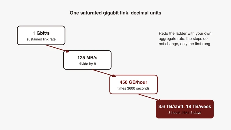
- 1 Gbit/s is 1,000,000,000 bits per second.
- Divide by 8 bits per byte: 125,000,000 bytes per second, which is 125 MB/s.
- Multiply by 3,600 seconds in an hour: 450,000,000,000 bytes, which is 450 GB per hour.
- Multiply by an eight-hour shift: 3,600 GB, which is 3.6 TB per shift.
- Multiply by five shifts: 18,000 GB, which is 18 TB per week.
The ladder runs at any rate. Two saturated directions of a 100BASE-T1 link are 200 Mbit/s, or 25 MB/s, or 90 GB per hour. A 500 kbit/s CAN bus at full load is 62,500 bytes per second, or 225 MB per hour. That is the bus rate, not the written rate. Encapsulated, a bus of thousands of small frames per second costs several times that on disk, which is why the per-frame overhead has to be measured on your own chain rather than estimated. Even so, CAN does not drive the sizing once a camera is in the rig.
A raw camera worked end to end
This is uncompressed sensor arithmetic, not a product figure: what an unencoded camera stream costs if you record it raw.
- 1920 by 1080 pixels is 2,073,600 pixels per frame.
- At 12 bits per pixel: 24,883,200 bits per frame.
- At 30 frames per second: 746,496,000 bits per second, about 746.5 Mbit/s.
- Divide by 8: 93,312,000 bytes per second, about 93.3 MB/s.
- Multiply by 3,600: 335,923,200,000 bytes, about 336 GB per hour.
That is roughly three quarters of a gigabit link, and resolution, bit depth and frame rate each scale it linearly. Uncompressed links at this rate run over SerDes rather than Ethernet, which is why the raw figure above is a sizing bound rather than something you will see on a capture port; compressed camera streams over automotive Ethernet are what a logger fed from the network actually records.
Multi-sensor rigs, and the compression decision
Four such cameras is 4 times 93.312, or 373.25 MB/s, about 1.34 TB per hour, before radar, lidar, buses or encapsulation overhead. That number forces the compression conversation. Compressing on the logger cuts the write rate and the media you carry, at the cost of processing inside a box already meeting a deadline, and lossy video compression removes information some later analysis will want. Compressing after offload keeps the recording as captured, but you needed the rate and capacity in the vehicle. Decide per stream.
The ladder
Decimal units throughout, an eight-hour shift, five shifts per week.
| Aggregate rate | Bytes per second | Per hour | Per shift | Per week |
|---|---|---|---|---|
| 100 Mbit/s | 12.5 MB/s | 45 GB | 360 GB | 1.8 TB |
| 200 Mbit/s | 25 MB/s | 90 GB | 720 GB | 3.6 TB |
| 500 Mbit/s | 62.5 MB/s | 225 GB | 1.8 TB | 9 TB |
| 1 Gbit/s | 125 MB/s | 450 GB | 3.6 TB | 18 TB |
| 2 Gbit/s | 250 MB/s | 900 GB | 7.2 TB | 36 TB |
| 3 Gbit/s | 375 MB/s | 1.35 TB | 10.8 TB | 54 TB |
| 5 Gbit/s | 625 MB/s | 2.25 TB | 18 TB | 90 TB |
Headroom: why sizing to the average rate loses the interesting event
Traffic bursts, so a path sized to the average has no margin, and drops arrive when activity peaks, which is the moment you were recording for. Size to the peak sustained rate you can justify, add the encapsulation overhead you measured, and treat the result as a floor.
Triggers and filters: not recording everything
At some rates, recording everything for the whole drive is not a decision anyone gets to make.
Ring buffer plus event trigger, the standard pattern
Continuous ring buffering plus a trigger that promotes a window to permanent storage: everything recent is in hand, only what matters is kept. The mechanics are familiar from bench tooling, where dumpcap’s multiple-files mode switches file on a value in seconds, kilobytes or packets and forms a ring buffer of a given number of files. A vehicle logger runs the same idea against a trigger input.
Signal-level triggers versus frame-level filters
A frame-level filter decides what gets written, cheaply and bluntly. A signal-level trigger decides when something interesting happened, which needs the logger to interpret the payload, so it depends on the database or description file loaded into it matching what the ECU emits. Ask which buses a candidate triggers on at signal level, and what it needs loaded.
Why over-filtering destroys post-hoc analysis you have not thought of yet
A filter is a decision made before you know the question, and the commonest regret in vehicle logging is a recording that answers the question from the planning meeting and nothing else. Where the rate allows it, record broadly and filter offline. Where it does not, keep the filter list beside the recording, so a future engineer knows what is absent rather than concluding it never happened.
Marking events during the drive so you can find them later
A marker input, a button, or an event injected into the stream turns “somewhere in the third hour” into a seek. It is the cheapest feature on the list and the one most often left unconfigured.
After the drive: offload and the offline toolchain
Offload paths: removable media, wired transfer, wireless
Removable media moves terabytes at the speed of a person carrying it: fast, manual, easy to mishandle. Wired transfer keeps the media in the box and needs the vehicle back at a bay. Wireless suits fleet-scale selected signals rather than validation-scale raw capture. Match the path to the daily volume you computed, not to the interface list.
File formats, and whether your analysis tools read what the logger writes
The logger may store the encapsulated stream as received, or convert it. Those are different products to live with, and only one opens directly in the tool your team already uses. Ask for the file format by name and confirm your scripts read it before hardware ships: our capture encapsulation article covers how format versions and field names have moved.
Correlating buses, sensors and video on one timeline
Correlation is a timestamp problem before it is a tooling problem. One encapsulated stream from one capture module gives one time base by construction; a logger plus a separate video recorder gives two, and aligning them afterwards is a project. A distributed time base is only as good as the synchronisation behind it, and our gPTP troubleshooting article covers what has to work first. Both formats carry a flag saying whether the timestamp was synchronised: check it before any number is quoted as a measurement.
Data governance: personal data in location, cabin and camera streams
This is a question for your data protection owner, and engineering’s job is to raise it before the drive rather than after the recording exists. India’s Digital Personal Data Protection Act, 2023, published as Act No. 22 of 2023 with assent on 11 August 2023, defines personal data as any data about an individual who is identifiable by or in relation to such data, and applies to the processing of digital personal data within the territory of India where it is collected in digital form, or collected on paper and digitised afterwards, and it reaches processing outside India where that processing is connected with offering goods or services to people in India. A validation recording can hold several things that plausibly meet that definition: location traces that identify a driver’s routine, cabin audio and video, exterior footage containing faces and number plates.
Naming the obligations is as far as this article goes. Section 4 permits processing only for a lawful purpose, with consent or as a certain legitimate use. Section 5 requires a notice accompanying or preceding a request for consent. Section 6 requires consent to be free, specific, informed, unconditional and unambiguous, with a right to withdraw it. Section 8 requires reasonable security safeguards against a personal data breach, erasure once the specified purpose is no longer served unless law requires retention, and published contact details for someone who can answer questions.
Four questions for whoever owns this in your organisation, in writing, before the first drive. Which streams contain personal data. What is the lawful basis for recording them. How long may recordings be retained, and who erases them. What happens when a recording goes to a supplier or an OEM customer.
Shortlisting: the questions that separate the boxes
The checklist
Take this to every quotation and require written answers.
| Criterion | The question | Why it separates candidates |
|---|---|---|
| Aggregate rate | Sustained write rate across all streams at once, measured how? | A per-interface figure hides the total |
| Interfaces | Which buses natively, which via an external capture module? | One product or three |
| Timestamp source | What clock, how synchronised, what does the flag show on loss? | Every timing conclusion rests on it |
| Buffering | How much buffer in front of the media, and how deep is the pre-trigger window, in seconds at our rate? | Absorbs bursts and rotation stalls |
| Storage | Capacity in decimal units, media type, and on overload: silent drop or marked gap? | Silent drop makes analysis unfalsifiable |
| Offload | Which paths, which file format out, how long for our daily volume? | Decides whether your toolchain reads it |
| Environmental rating | Temperature, vibration and ingress where it will actually be mounted | A bench-rated box in a boot |
| Management | Configuration read back as a file and version controlled? | Reproducibility, not convenience |
Where a logger stops and a HIL rig starts
A logger observes and records. A hardware-in-the-loop rig stimulates: it generates traffic, injects faults and closes the loop around the device under test. Replaying a recording is sometimes treated as stimulation, which works for simple cases and breaks the moment the ECU expects a response that depends on what it just sent. If your test plan says inject, simulate or respond, you are in a different category.
Sourcing and support in India
Capture and logging equipment is largely imported, so the schedule that matters is the one ending with a working bench, GST invoicing and paperwork included. And when a logger drops frames in week three, the useful support is an applications engineer who will open your capture inside your working hours.
Where GSAS fits
GSAS Micro Systems is an engineering partner, and on data logging the useful conversation happens before the purchase order. Two things decide the outcome: the aggregate rate you will actually generate, measured rather than estimated, and where in the chain you can afford to lose frames. Most shortlists resolve once those numbers exist, and some resolve to equipment already on the bench.
A rate budget and storage sizing review is a working session. We go through the capture path with you, count the streams, apply the arithmetic above to your numbers including the encapsulation overhead measured on your own chain, and tell you which checklist questions your quotations have not answered. Our applications engineers work in IST, so a bench session lands inside your working day, and the teams we work with sit in Bengaluru, Pune, Chennai and Hyderabad.
Start with the automotive Ethernet capability page, then request a scoped conversation describing your buses, your sensor streams and how long you need to record. Where your existing setup already meets the budget, that is the answer you get.
References
- India Digital Personal Data Protection Act, 2023 (No. 22 of 2023), official Gazette text, Ministry of Electronics and Information Technology (assent 11 August 2023; sections 2(t), 3, 4, 5, 6, 8 and 17(2)(b)): https://www.meity.gov.in/static/uploads/2024/06/2bf1f0e9f04e6fb4f8fef35e82c42aa5.pdf
- libpcap
pcap_statsmanual page, tcpdump.org (ps_recv,ps_drop, platform caveats,ps_ifdrop): https://www.tcpdump.org/manpages/pcap_stats.3pcap.html - Wireshark
dumpcapmanual page (multiple-files ring buffer criteria;-Bcapture buffer size): https://www.wireshark.org/docs/man-pages/dumpcap.html - Wireshark display filter reference,
tecmp(tecmp.counter, 16-bit unsigned;tecmp.dev_flags.device_overflow, boolean): https://www.wireshark.org/docs/dfref/t/tecmp.html - ASAM CMP standard page, ASAM e.V. (capture module to data sink model; version 1.1.0, 26 January 2026): https://www.asam.net/standards/detail/cmp/
- Wireshark wiki, CaptureSetup/Ethernet (the monitoring port must be at least as fast as the monitored port): https://wiki.wireshark.org/CaptureSetup/Ethernet
- OPEN Alliance TC10 sleep and wake-up specifications, 100BASE-T1 and 1000BASE-T1 (objectives: global network wake-up including link start-up in under 250 ms), via the OPEN Alliance public specification hub: https://www.opensig.org/
Also appears in:
Building for Automotive & Mobility?
Talk to our application engineers for personalized tool recommendations.