Energy Profiling IoT Devices: From Sleep Current to Peak Transmission

An IoT device’s battery life is not determined by a single current number. It is determined by the time-weighted sum of every operating state the device passes through, deep sleep, light sleep, sensor acquisition, data processing, radio transmission, radio reception, and every transition between them. Miss any one of these states, or mismeasure it, and the battery life estimate will be wrong. Sometimes catastrophically wrong.

This article breaks down the anatomy of an IoT power budget, explains why conventional instruments fail to capture it accurately, and describes the measurement workflow that produces reliable battery life predictions, using continuous high-resolution sampling to capture every microamp and every microsecond of the device’s operating cycle.

Anatomy of an IoT Power Budget

A typical low-power IoT sensor node, a temperature/humidity sensor reporting to a LoRa gateway every 15 minutes, for example, cycles through distinct operating states with dramatically different current consumption.

Deep sleep is the lowest power state, where the MCU core is powered down and only a real-time clock (RTC) or low-power timer maintains the wakeup schedule. Modern ultra-low-power MCUs draw 100 nA to 2 uA in this state, depending on RAM retention requirements and peripheral configuration. Since the device spends 99%+ of its time in deep sleep, this current dominates the average power budget despite being the smallest instantaneous value. Wake and initialization occurs when the RTC alarm fires and the MCU begins resuming from deep sleep. The MCU powers up its oscillators, restores core registers, and initializes peripherals. This phase typically draws 1-10 mA for 1-50 ms, depending on the MCU architecture and the oscillator settling time (crystal oscillators take longer than RC oscillators). Sensor acquisition powers up external sensors, waits for their settling time, triggers a measurement, and reads the result. Current consumption depends heavily on the sensor type: a temperature sensor might draw 100 uA for 10 ms, while a particulate matter sensor might draw 100 mA for several seconds. The sensor’s power-up settling time is often the dominant factor, many sensors require 10-100 ms of stabilization before their first valid reading. Data processing runs the application logic: filtering sensor data, applying calibration, formatting a packet, computing a checksum. This phase runs at the MCU’s active current (typically 5-50 mA depending on clock frequency and voltage) but is usually brief, a few hundred microseconds to a few milliseconds for simple sensor applications. Radio transmission is typically the highest-current phase. A LoRa radio transmitting at +22 dBm draws 120-140 mA. A BLE radio transmitting an advertisement draws 5-15 mA for 1-3 ms. A cellular modem transmitting an LTE-M packet can draw 200-500 mA for hundreds of milliseconds. The peak current and duration together determine the energy cost per transmission. Radio reception follows transmission in protocols that require acknowledgment. The device listens for a response from the gateway, drawing the radio’s receive current (typically 5-15 mA for LoRa, 5-10 mA for BLE) for a receive window that may last milliseconds to seconds. In LoRaWAN, the receive windows (RX1 and RX2) are the second-largest energy consumers after the transmission itself.

Why Multimeters Cannot Capture This

A benchtop multimeter on its DC current range might display “0.15 mA” for a device that is actually cycling between 200 nA deep sleep and 130 mA transmission bursts. The multimeter’s reading is some weighted average of these states, filtered through the meter’s bandwidth and display update rate, and it tells the engineer almost nothing useful about the actual power budget.

The fundamental problem is bandwidth and dynamic range. A multimeter’s current measurement has a bandwidth of perhaps 1-10 Hz and a dynamic range of 3-4 decades on any single range. An IoT device’s current profile has features at microsecond timescales and spans 6-9 decades of current range. The multimeter smooths, averages, clips, and distorts the actual current waveform beyond recognition.

An oscilloscope with a current shunt can capture fast transients, but it faces a different problem: dynamic range. A shunt resistor that provides good voltage resolution at 200 nA (requiring a large resistance value) drops excessive voltage at 130 mA (causing the device to malfunction or the oscilloscope to saturate). Switching between shunt values means switching measurement ranges, which creates gaps in the data and requires the engineer to stitch together multiple captures.

Joulescope: Continuous 2 Msps Across 9+ Decades

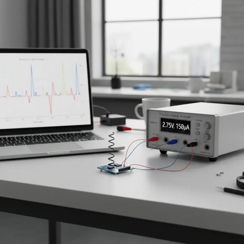
The Joulescope JS220 solves both problems simultaneously. Its Enwavify autoranging technology switches between optimized shunt resistors in 1 microsecond, continuously selecting the shunt that provides the best resolution for the instantaneous current. The 2 Msps 16-bit simultaneous ADCs capture current and voltage with 300 kHz bandwidth and 0.5 nA resolution, spanning from deep-sleep nanoamps to +/-10 A peak current without any gaps, dead zones, or range-switching artifacts.

The result is a continuous, high-resolution record of exactly what the device draws at every point in its operating cycle. Deep sleep at 350 nA, the RTC wakeup transient at 2 mA for 800 us, the sensor power-up at 1.5 mA for 15 ms, the LoRa transmission at 128 mA for 52 ms, the two receive windows at 12 mA for 1 second each, all captured in a single, uninterrupted acquisition.

The 20 mV maximum burden voltage is critical for accurate profiling. Some current measurement approaches insert large shunt resistors (100 ohms or more) that drop significant voltage when the device draws milliamps or amps. This voltage drop changes the supply voltage seen by the device, which changes its behavior, potentially altering the operating point of voltage regulators, changing the radio’s output power, or preventing the MCU from entering its lowest power state.

The JS220’s 20 mV burden ensures the device operates as it would in the final product.

Average Power vs. Peak Power

Engineers new to IoT power profiling sometimes focus exclusively on peak current, the maximum current during radio transmission. Peak current matters for battery selection (the battery must be able to source the peak current without excessive voltage droop) and for power supply design (the regulator must maintain regulation during peak loads). But peak current is almost irrelevant for battery life estimation.

Battery life is determined by average current, the total charge consumed divided by the total time. For a device that sleeps for 15 minutes, wakes for 200 ms to sense and transmit, and then sleeps again, the average current is dominated by the sleep current even though the active current is six orders of magnitude higher.

Here is a concrete example. A sensor node with these operating characteristics:

• Deep sleep: 500 nA for 899.8 seconds (14 minutes 59.8 seconds)
• Active cycle: 50 mA average for 200 ms (sensor + process + transmit + receive)

The charge per cycle is: (500 nA x 899.8 s) + (50 mA x 0.2 s) = 0.45 uAh + 2.78 uAh = 3.23 uAh

Average current = 3.23 uAh / (900 s / 3600 s/h) = 12.9 uA

On a 2600 mAh AA lithium battery: 2600 / 0.0129 = 201,550 hours = 23 years (exceeding the battery’s shelf life).

Now, what if the firmware has a bug that prevents deep sleep, keeping the MCU in light sleep at 5 uA instead of 500 nA?

Charge per cycle: (5 uA x 899.8 s) + (50 mA x 0.2 s) = 1.25 uAh + 2.78 uAh = 4.03 uAh

Average current = 16.1 uA. Battery life = 18.4 years. The difference is measurable, about 20%, but both numbers still seem acceptable.

But increase the sleep current to 50 uA (a common scenario when a peripheral is accidentally left powered):

Charge per cycle: (50 uA x 899.8 s) + (50 mA x 0.2 s) = 12.5 uAh + 2.78 uAh = 15.28 uAh

Average current = 61.1 uA. Battery life = 4.9 years. Now the sleep current dominates and cuts battery life by 4x.

These calculations show why accurate sleep current measurement, at the nanoamp level, determines whether the battery life estimate is trustworthy.

Energy Per Transaction

Beyond average current, energy-per-transaction is the metric that connects firmware behavior to battery cost. A “transaction” is one complete operating cycle: wake, sense, process, transmit, receive, sleep. The energy consumed by one transaction, measured in microjoules or millijoules, tells the engineer exactly what each sensor reading or data upload costs in battery capacity.

The Joulescope UI computes energy over user-defined time windows, making it straightforward to isolate a single transaction and measure its energy cost. The Python API enables scripted measurement that automatically triggers on a wake event, captures the complete transaction, and reports the energy consumed, enabling automated regression testing that catches firmware changes that increase energy-per-transaction.

Energy-per-transaction analysis also reveals optimization opportunities. If the radio receive window accounts for 60% of the transaction energy, optimizing the receive window duration (or switching to a protocol with shorter acknowledgment windows) has a far greater impact on battery life than optimizing the sensor acquisition phase.

Common Firmware Pitfalls

Years of power profiling with Joulescope across hundreds of IoT designs have revealed recurring firmware bugs that destroy battery life. These bugs share a common characteristic: they are invisible to functional testing and often invisible to multimeter-based power measurement.

Peripherals left enabled during sleep. The most common bug. An SPI bus clock left running, a UART receiver left enabled, or an ADC left in standby mode can add 10-100 uA to the sleep current. The fix is trivial, disable every peripheral before entering sleep, but the bug is invisible without nanoamp-resolution measurement. Oscillator not switching to low-power source. Many MCUs use a high-frequency crystal oscillator for active operation and an internal low-power RC oscillator for timekeeping during sleep. If the firmware fails to switch oscillator sources before entering sleep, the high-frequency oscillator continues running, drawing milliamps instead of nanoamps. GPIO pins floating or configured as inputs without pull-ups/pull-downs. A floating input pin can oscillate, causing the input buffer to draw dynamic current. Configuring unused pins as outputs driven low (or as analog inputs with the digital input buffer disabled) eliminates this leakage. Voltage regulator not entering low-power mode. External voltage regulators often have an enable pin or a low-power mode selection pin. If firmware does not assert these signals before sleep, the regulator continues operating in full regulation mode, consuming its active quiescent current. Unexpected wake events. A misconfigured interrupt, a noisy sensor output, or an incorrect wake timer period can cause the device to wake frequently, perhaps every 100 ms instead of every 15 minutes. Each unnecessary wake costs a full active cycle’s worth of energy. Joulescope’s continuous capture makes these unexpected wakes immediately visible as current spikes in the time-domain view.

Battery Life Estimation Workflow

The complete workflow from Joulescope measurement to battery life estimate follows these steps:

1. Connect the JS220 in series with the device’s power supply, using the shortest practical cables.
2. Capture several complete operating cycles (wake-sense-transmit-sleep-wake) with sufficient duration to establish the sleep current baseline.
3.

Measure the average current over an integer number of complete cycles.
4. Derate the battery capacity for temperature, age, and self-discharge (typically 70-80% of nominal for a conservative estimate).
5. Calculate: Battery life = Derated capacity / Average current.
6.

Validate by running a multi-day capture and confirming that the average current remains consistent.

Get Joulescope Power Profiling Support from GSAS India

GSAS Micro Systems is the authorized Joulescope partner in India, providing the JS220 and JS220+ energy analyzers with INR invoicing, evaluation unit programs, and hands-on power profiling methodology workshops for engineering teams. Whether you are profiling a BLE sensor for a wearable, a LoRa node for smart agriculture, or a cellular tracker for fleet management, our applications engineering team provides measurement setup guidance, fixture design, Python API training for CI/CD integration, and result interpretation support. Contact us from Bengaluru, Chennai, Hyderabad, Delhi NCR, Mumbai, or Pune.