In short
Hardware trace records when interrupts, tasks and runnables actually executed on the target, without stopping the core, so you can measure interrupt latency, task jitter and observed execution times on real hardware. Measurement gives you a distribution and an observed maximum, not a guaranteed upper bound. AUTOSAR's own timing analysis guidance says upper bounds come from static analysis, so use trace to validate timing behaviour and static analysis to bound it.
Most of the bugs that escape an automotive ECU programme are not logic bugs. They are timing bugs: an interrupt handled late under one specific bus load, a task that overruns once every few hours, a runnable that blows its budget only when a diagnostic session is open. They pass every breakpoint-driven debug session because a halted core has no timing to observe.
Hardware trace is the tool that turns timing from a guess into a measurement. This article covers three questions Indian AUTOSAR teams ask of it, interrupt latency, task jitter and execution time, and is explicit about the line where measurement stops being evidence and static analysis has to take over.
Why timing needs trace, not breakpoints
A breakpoint stops the core, and with it everything you wanted to time. Software timestamps, toggled GPIO pins and logging calls work, but each one adds code, and code changes timing: the probe effect. Trace avoids both problems. The trace hardware in the chip records program flow while the core runs at full speed, and the debugger reconstructs what happened, and when, from the stream and the program image.
On Arm cores the source is the ETM, which can add timestamps and, in cycle-accurate mode, cycle counts to the trace stream. On Cortex-M devices the DWT unit adds exception trace and PC sampling, which Arm’s Keil documentation describes, and those are often enough for a first look at interrupt behaviour over a single SWO pin. The off-chip trace explainer covers how each kind of trace leaves the chip.
Interrupt latency
Interrupt latency is the time from the event that raises an interrupt to the point where its handler does the work that matters. Trace measures it directly: find the exception entry in the trace, find the handler instruction you care about, and subtract timestamps.
Three practices make the number trustworthy:
- Measure many occurrences, under realistic load. Latency depends on what the core was doing when the interrupt arrived: a higher-priority handler, a critical section with interrupts masked, a long instruction. One measurement tells you almost nothing.
- Define the end point by the requirement. “Handler entry” and “actuator command written” are different numbers. Measure the one your requirement names.
- Report a distribution. Minimum, typical and maximum observed, plus how many occurrences and under which load. A latency histogram is far more useful to a reviewer than a single figure.
Task and runnable jitter
In an AUTOSAR Classic ECU, runnables are mapped to OS tasks that are activated periodically or by events. Jitter is the variation in when a task actually starts, or finishes, relative to when it should.
Trace gives you two ways to see it:
- From program flow. Instruction trace shows when the OS dispatcher ran and when each task entry function executed. Task start times and jitter fall out of the trace without adding hooks to the build. A debugger that is aware of your OS can present this as a task timeline.
- From instrumentation. Tools such as SEGGER SystemView record OS events through software hooks and stream them to the host. That works with any debug probe, at the cost of adding recording code to the build. Our post on RTOS-aware debugging in Keil MDK covers the Keil side of OS awareness.
Both are legitimate. Program-flow trace is the stronger evidence when the question is “did adding observation change the timing?”, because nothing was added.
Execution time, and where WCET evidence comes from
This is where teams most often overclaim. Trace makes it easy to measure how long every runnable took across a test campaign, and it is tempting to call the longest observed time the worst-case execution time. It is not.
AUTOSAR’s own guidance is direct about this. The Recommended Methods and Practices for Timing Analysis and Design within the AUTOSAR Development Process groups timing methods into simulation, analytical calculation and measurement. It states that measurements can only provide average execution times or a distribution of execution times, and that static analysis techniques are employed to obtain an execution time upper bound. The same document warns that a static analysis tool can also produce wrong results when it is not configured correctly.
The practical consequence is a division of labour:
| Question | Measurement from trace | Static WCET analysis |
|---|---|---|
| What did the code actually do on this hardware? | Yes, directly | No, it models the hardware |
| What is the longest execution observed in testing? | Yes | Not applicable |
| What is a safe upper bound on execution time? | No | Yes, if correctly configured |
| Is the static model consistent with reality? | Yes, as a cross-check | Needs measurement to check |
| Which paths did the tests exercise? | Yes, through coverage | Not applicable |
Used together, they are strong evidence. The trace shows real behaviour and which paths were exercised, and the static bound covers the paths and states the tests did not reach. The coverage side of that story is in trace-based code coverage as ISO 26262 and DO-178C evidence.
Tie every measurement to an AUTOSAR timing constraint
Timing evidence is only useful if a reviewer can see which requirement it supports. AUTOSAR’s Specification of Timing Extensions (TIMEX) defines how timing requirements are written into the system description. It includes latency constraints on event chains, where one event is understood to cause the next, and execution time constraints on executable entities.
Map each trace measurement to one of those constraints: this end-to-end latency figure supports that event-chain constraint, this execution time distribution supports that runnable’s budget. Measurements that are not tied to a constraint are debugging data, not evidence.
Timing in a functional safety argument
In an ISO 26262 programme, timing also matters for freedom from interference. Public teaching material on ISO 26262 lists timing and execution, alongside memory, as a dimension of interference between software elements, addressed with mechanisms such as scheduling, execution budgets and watchdogs. Trace can show, on real hardware, that a budget mechanism actually contained an overrunning task. Our ISO 26262 compliance page covers how GSAS maps tools to the standard’s verification activities. ISO 26262 is a paywalled standard, so this article quotes no clause numbers from it.
A practical workflow
- List the timing constraints the ECU must meet, by name, from the TIMEX description or the requirements.
- Bring up trace on a development board that represents production timing: same clocks, same memory configuration, same compiler options.
- Run the test campaign with trace capture and timestamps enabled, under realistic bus and diagnostic load.
- Extract interrupt latencies, task start times and runnable execution times, and report distributions per constraint.
- Compare observed maxima against static WCET bounds where you have them, and investigate any measurement that comes close.
Tools GSAS supplies today
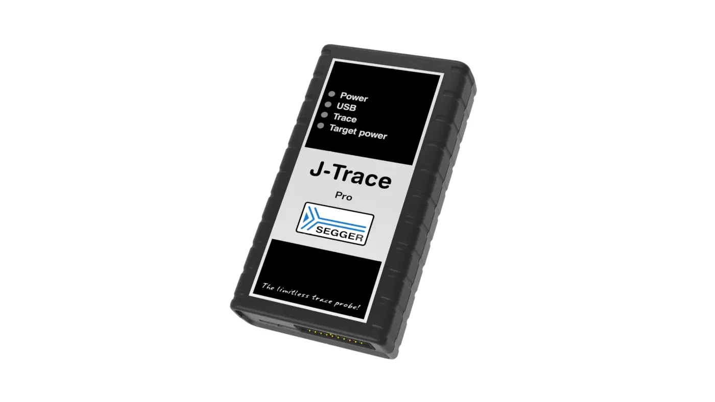
- Arm Cortex-M, Cortex-A and Cortex-R, and RISC-V: SEGGER J-Trace PRO with Ozone. SEGGER describes Ozone’s integrated performance analysis tools as including instruction trace, code profiling and code coverage, with visual timelines.
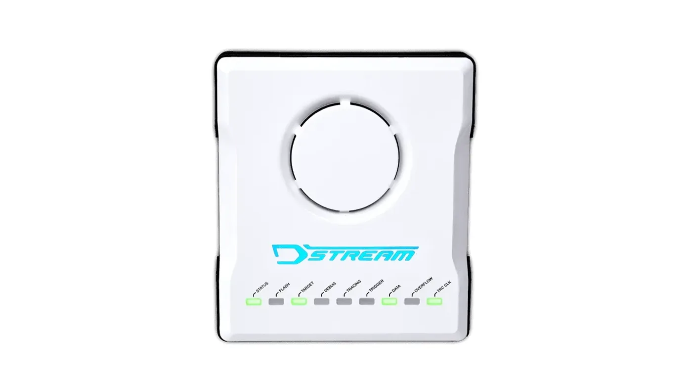
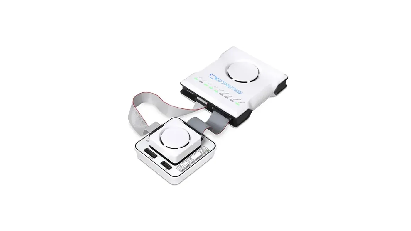
- Multicore Arm: Arm Development Studio with DSTREAM-ST or DSTREAM-PT.
- Instrumentation-based RTOS timing: SEGGER SystemView.
For timing analysis on multicore AURIX/TriCore and RH850 ECUs, talk to our FAE team about the right probe for your device and trace interface.
Where GSAS fits
GSAS Micro Systems supplies trace probes, debuggers and timing tools in India with INR quotations and local application engineering. Our engineers in Bengaluru, Pune, Chennai and Hyderabad help AUTOSAR teams set up trace on representative hardware and turn measurements into evidence tied to named constraints. Teams in Mumbai and Delhi NCR are supported on site and remotely.
Related reading
- Multicore debug on AURIX, RH850 and Cortex-R52
- Non-intrusive debug of safety ECUs on production silicon
- SEGGER J-Trace PRO streaming trace
- Choosing debug and trace tools for Indian automotive Tier-1s
References
- AUTOSAR, Specification of Timing Extensions for Classic Platform (R24-11, document 411): https://autosar.org/fileadmin/standards/R24-11/CP/AUTOSAR_CP_TPS_TimingExtensions.pdf
- AUTOSAR, Recommended Methods and Practices for Timing Analysis and Design within the AUTOSAR Development Process (document 645): https://www.autosar.org/fileadmin/standards/R22-11/FO/AUTOSAR_TR_TimingAnalysis.pdf
- AUTOSAR, Recommended Methods and Practices for Timing Analysis and Design, R4.1.3 edition: https://www.autosar.org/fileadmin/standards/R4.1.3/CP/AUTOSAR_TR_TimingAnalysis.pdf
- FAU Erlangen-Nuremberg, lecture material on ISO 26262 freedom from interference: https://www4.cs.fau.de/Lehre/SS18/V_VEZS/Skript/X-Industrievortrag_a4.pdf
- Arm, Keil Application Note KAN339 (Cortex-M trace sources): https://documentation-service.arm.com/static/61f93536fa8173727a1b72ab
- SEGGER, Ozone debugger: https://www.segger.com/products/development-tools/ozone-j-link-debugger/
- SEGGER, J-Trace product family: https://www.segger.com/products/debug-probes/j-trace/
Also appears in:
Building for Automotive & Mobility?
Talk to our application engineers for personalized tool recommendations.
More from SEGGER
View all →
Choosing Debug and Trace Tools for Indian Automotive Tier-1s
13 Nov · 11 min
Multicore Debug on AURIX, RH850 and Cortex-R52 in India
13 Nov · 11 min
Non-Intrusive Debug of Safety ECUs on Production Silicon
13 Nov · 10 min
Off-Chip Trace Explained: ETM, Serial Trace, Trace Buffers
13 Nov · 10 min
Emulation vs FPGA Prototyping vs Simulation for SoC Teams
13 Nov · 8 min
GW Instek LCR-7000 and GPM-8340: New in India for 2026
13 Nov · 6 min